The attributes in this section define the basic characteristics of the fluid container.
Defines the size of the fluid container in world space units.
Boundary X, Y, Z
The boundary attributes control the way the solver treats property values at the boundaries of the fluid container.
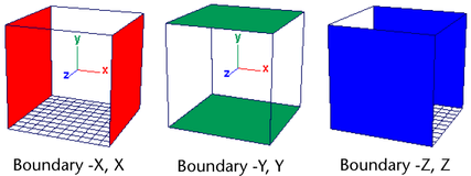
For each boundary select one of the following boundary definitions:
(For 2D containers only.) Turn this option on to draw a 2D surface as a height field rather than a flat plane. This is useful for generating effects such as foam on a cappuccino or boat wakes.
This option affects both surface shaded renders as well as normal volume renders. (Remember that 2D fluids are really 3D fluids. The dynamic grid and textures are defined in 2D and projected onto the 3D volume.)
When Use Height Field is on, Opacity is reinterpreted to mean the height of a uniform opacity. This offset is in the Z axis coming out of the fluid. An Opacity value of 0.0 means a height of 0 and an Opacity value of 1 means the fluids fills up to the maximum Z boundary. The Z size of the 2D fluid is defined by the Size attribute.
The playback speed for Surface Render of 2D fluids is much faster if Use Height Field is on.
For each of the fluid properties, select which method to use to populate the fluid container with property values. For each property, you can scale the values in the container to uniformly increase or decrease them. See Contents Details.
Density/Velocity/Temperature/Fuel
Select one of the following options:
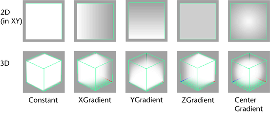
Uses the selected gradient to populate the fluid container with property values. Gradient values are predefined in Maya without the use of a grid. Gradient values are used in calculations for dynamic simulations but the values cannot change because of the simulation. They render more quickly than grid values because no calculations are required for simulation.
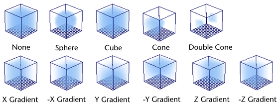
Density/Velocity/Temperature/Fuel Gradient
(Available when the previous method is set to Gradient.)
Select which predefined set of values you want to place in the container:
Color Method
Color displays and renders only where Density is defined. Select which method to use to define color.
For Static and Dynamic Grids, the default grid color is green/brown (close to RGB 0.4 0.4 0.3) to minimize fringing where any colored Density you add meets voxels with no Density values. If this is not an acceptable grid color, flood the color grid with the color you want and set it as your initial state, see Flood a container with values and Fluids initial state.
The Display options affect how the fluid displays in the scene view. They do not affect the final rendered image.
Defines which fluid properties display in the fluid container when Maya is in shaded display mode. If Maya is in wireframe mode, the Wireframe Display options apply to the selected property.
Select Off to display nothing in the fluid container when in shaded display mode.
Select As Render to display the fluid as close as possible to the final software render.
Isolating the display of a specific property of the fluid (for example, Fuel) is particularly useful when painting the property with the Paint Fluids Tool or adjusting settings for it. Tweak the Opacity Preview Gain to map the selected property to a useful range of opacity in the grid.
For display options combining Density with another property (for example, Density And Temp), color differentiates the two properties. If the second attribute is not color, then you get a built-in ramp (with blue, red and yellow) that maps the interval 0-1; where there is no density, there is no information about the second attribute.
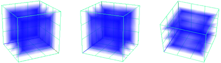
Defines the number of slices displayed per voxel when Maya is in shaded display mode. A slice is a display of values on a single plane. Higher values produce more detail but reduce the speed of the screen draw. The default is 2. The maximum value is 12.
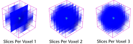
The orientation of the slices is determined by the voxel most aligned with the view plane.
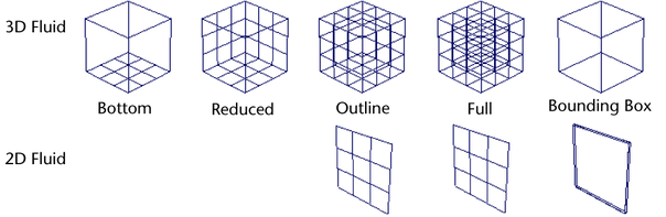
Boundary Draw
Defines how the fluid container displays in 3D views. The grid corresponds with the Resolution settings.
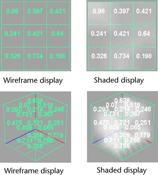
Displays numeric values for the selected property (Density, Temperature, or Fuel) in each voxel of a Static or Dynamic Grid. The numbers that display represent the values before the Scale is applied. For example, if the Density value in a voxel is 0.2 and the Density Scale is 0.5, the number that displays in the voxel is 0.2, not 0.1. No numeric values display when this option is set to Off or when the Contents Method for the selected property is set to Gradient.
Numeric Display can be used in both shaded and wireframe display modes.
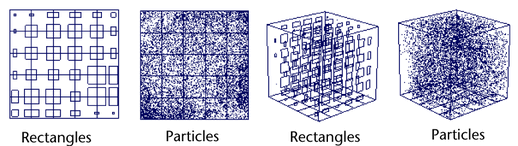
Wireframe Display
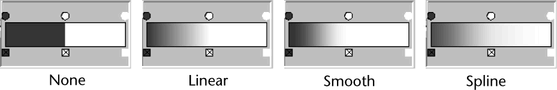
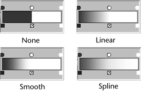
If the Contents Method is set to Gradient for the property selected for Shaded Display, this option defines how to represent the opacity of the property when Maya is in wireframe display mode.
If Contents Method is set to Static or Dynamic Grid for the property selected for Shaded Display, this option defines how to represent the values of the property when Maya is in wireframe display mode.
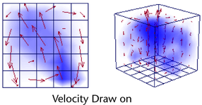
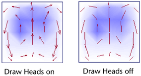
Defines the length of the velocity vectors (a factor applied to the magnitude of the velocity). The larger the value, the longer the velocity segments or arrows. For simulations with very low force, the velocity field might be very small in magnitude. In this case, increasing the value will help to visualize the velocity flow.
To simulate flow for a fluid property, the Contents Method for that property must be set to Dynamic Grid and Velocity cannot be Off. During simulation, the values in the container are solved using the Navier-Stokes fluid dynamics equations (solvers) and replaced with the new values to create the fluid motion. Use the attributes in this section to define the information used by the solvers.
The Gravity setting is a built-in gravitational constant that simulates the gravitational attraction of the mass of the world in which the simulation is occurring. Negative values cause a downward pull (relative to the world coordinate system).
If Gravity is zero, Density Buoyancy and Temperature Buoyancy have no effect
Viscosity represents the resistance of the fluid to flow, or how thick, and non-liquid the material is. When this value is high, the fluid flows like tar. When this value is small, the fluid flows more like water.
(When Viscosity is 1, the material Reynolds Number is 0; when it is 0, the Reynolds Number is 10000. The Reynolds Number is a parameter used in solving the fluid dynamics equations that is proportional to the viscosity of the fluid.)
High Detail Solve
This option may reduce diffusion of density, velocity and other attributes during a simulation. For example, it may make fluid simulations appear much more detailed without increasing resolution, and allow the simulation of rolling vortices. Using High Detail Solve is ideal for creating effects such as explosions, rolling clouds and billowing smoke.
Pushes around other grid values, like density, but it also pushes its own velocity values to new positions in the grid. There is much more detail in the flow, resulting in a simulation that is significantly more realistic. Since propagating velocity is much more computationally intensive than propagating scalar grid values like density, using this option doubles the simulation computation time.
Grid Interpolator
Select which interpolation algorithm to use to retrieve values from points within a voxel grid.
Use a hermite curve to interpolate the fluid. This method causes less diffusion than linear, but makes the simulation run several times more slowly, especially when the fluid is colliding with geometry. Use hermite if you want Friction to be computed by the solver at the boundaries. (Use this option with the Velocity Only High Detail Solve method—while it is slower, it can yield high-quality results. Do not use this option with the All Grids Except Velocity or All Grids options.)
Sets the frame after which the fluid simulation will start. The default is 1.0. Nothing will play back for this object prior to this frame. You could use this attribute to delay the effect of a field on a fluid until the frame of your choice.
The attributes in this section are specific to each fluid property.
Density represents the material property of the fluid in the real world. You could think of it as the geometry of the fluid. If you compare it to a normal sphere, the volume equivalent of the sphere’s surface is the distribution of the Density inside the container.
A 1-1 correspondence with Density and Opacity is not typically desirable. An Opacity of 1.0 corresponds with an infinite density in nature (even materials like gold let a little light through). If the Density Scale is 1.0, the Transparency is 0.5, and the Opacity Input Bias is 0, you have a 1-1 correspondence. Lowering the Transparency and/or increasing the Opacity Input Bias helps create a more natural correspondence.
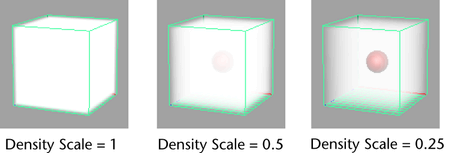
Multiplies the Density values in the fluid container (whether they are defined in grids, or defined by preset gradients) by the scale value. Using a Density Scale of less than 1 makes the Density appear more transparent. Using a Density Scale greater than 1 makes the Density appear more opaque.
In the following example, Density is set to Constant, which means it has a value of 1 throughout the fluid container. As you scale the Density values with a Density Scale less than 1, notice that the Density becomes less opaque and you can see the red ball contained in the fluid.
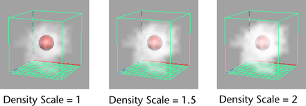
In the next example, Density is set to Dynamic Grid and the Density values are less than 1. As you scale the Density values with a Density Scale value greater than 1, notice that the Density becomes more opaque and the red ball contained in the fluid becomes more and more obscured by it.
Dynamic Grid only. Simulates a difference in mass density between the regions with Density values and the regions without. If the Buoyancy value is positive the Density represents a substance that is lighter than the surrounding medium, like bubbles in water, and will thus rise. Negative values cause the Density to fall.
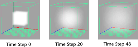
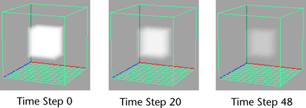
Defines the rate at which the Density gradually vanishes in a grid. At each time step Density is removed from each voxel (the Density value becomes smaller). In the following example, the Dissipation value is set to 1.
Fuel combined with Density defines a situation in which a reaction can take place. Density values represent the substance being reacted, and Fuel values describe the state of the reaction. Temperature can “ignite” Fuel to start a reaction (for example, an explosion effect). As the reaction progresses, the value of the fuel changes from unreacted (value 1) to fully reacted (value 0).
Fuel burns at temperatures greater than the Ignition Temperature.
Heat Released defines how much heat is released into the Temperature grid by a total reaction. This is how many reactions sustain themselves after an initial spark of ignition. The amount of heat added in a given step is proportional to the percentage of reacted material. You need to have the Temperature Method set to Dynamic Grid to use this option.
Select how you want the surface of the fluid to render.
Surface Render
Software render the fluid as a surface. The surface is formed by thresholding the Density values in the fluid container. Where the Density is greater than the Surface Threshold you are inside the medium, where it is less than this value you are outside the medium. (Surface Render combines blobby style surface rendering with normal soft volume style rendering.)
To see the surface in hardware display, Shaded Display must be set to As Render or the outMesh must have a connection. The surface location is determined by the current Opacity setting combined with the Surface Threshold.
Turn Soft Surface on to evaluate the changing Density based on the Transparency and Opacity attributes. The shadows tend to be softer and thin areas appear fuzzy.
For the light/normal shading Maya relaxes the angle of cutoff similar to the way Ambient Shade works in ambient lights.
For thick clouds like nuclear bombs, using Soft Surface can result in faster render times for a self shadowed effect, and unlike the Hard Surface render, you can have soft fuzzy areas.
Determines how close points sampled for a surface lie to the exact Surface Threshold Density. The tolerance value is defined relative to the Quality setting. The Quality determines the uniform step size, so that the actual distance this defines is equal to the step size Surface Tolerance.
Make the Quality setting just high enough so that you do not miss regions containing the surface. The render then further refines the surface using this tolerance.
If the Surface Tolerance is high then the surface will look dotty and of poor quality. Very low values result in longer render times and better quality.
In practical terms, Surface Tolerance helps better define the surface normal, because the local gradient used for the normal can vary quite a bit if the samples are not all close to the surface.
If your surfaces look grainy try lowering this value a bit (this is more critical when your Density is not smooth but very sharply defined, like with a thresholded texture, however a better solution is to make your Density smoother). If the graininess is due to missing the surface (that is, little holes) rather than noisy normals, then increasing the Quality is better.
The Environment ramp defines a simple sky to ground environmental reflection on a surface. The left of the ramp represents the top of the sky and the right represents the bottom.
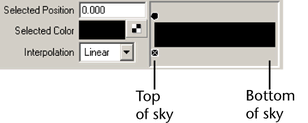
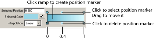
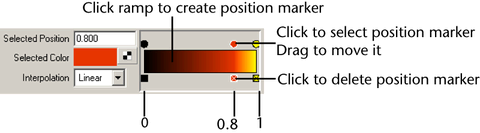
You define the reflection colors between the top and bottom of the sky by adding position markers to the ramp and changing the color at the markers.
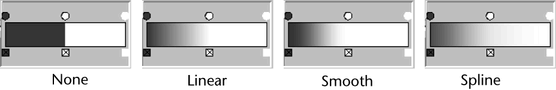
Interpolation
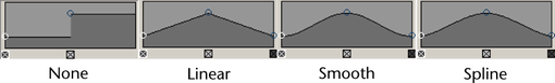
Controls the way colors blend between positions on the ramp. The default setting is Linear.
Index of refraction. This attribute affects how reflectivity changes with viewing angle. It makes use of Fresnel’s law. Materials with a low refractive index are generally only reflective at glancing angles. This is useful for a wet look or for water, because water has a lower refractive index than most solids. At a refractive index of 1.0 the material is considered to be the same as the medium, and theoretically there should be no specularity in this case (as with a cloud). However, for convenience, there is full specularity in this case (no view angle modulation).
The Output Mesh attributes allow you to control the resolution, smoothness, and speed of fluid to polygon mesh conversions.
Use this attribute to adjust the resolution of your fluid output mesh. Setting the Mesh Resolution to a low value allows you to quickly render fluid effects for partial previews. Higher output resolutions produce finer detail in the fluid, but increase rendering time. This attribute affects both the interactive display of surface style fluids, as well as the quality of the fluid to polygon mesh conversion.
Mesh Resolution does not affect the quality of the native fluid node render. Higher resolution values better resolve effects such as opacity texturing of the fluid. In addition, the higher resolution sampling takes advantage of the smooth render interpolation method when the method is enabled.
Turn this attribute on to make the normals on a fluid output mesh smoother. When on, the output mesh normals are created based on the direction of the opacity gradient within the fluid volume. This setting does not affect the interactive display of surface fluids, which uses the gradient normals. When turned off, the output mesh normals used for rendering are derived from the angles between triangles, which can result in relatively sharp edges where thin triangles are present.
Use the attributes in this section to apply built-in shading effects to the fluid.
Transparency combined with Opacity determines how much light can penetrate the defined Density. Transparency scales the single channel Opacity value. Using Transparency you can adjust the Opacity and also set its color.
You could adjust the Opacity of a fluid by moving the Transparency slider, ignoring all the other controls.
Controls the brightness of the glow (the faint halo of light around the fluid). Glow Intensity is 0 by default, so no glow is added to the fluid. As you increase the Glow Intensity, the apparent size of the glow effect increases.
Glow Intensity is different from the Incandescence attribute in two important ways:
The Color ramp defines a range of color values used to render the fluid. The particular colors selected from this range correspond with the values for the selected Color Input. Color Input values of 0 map to the color at the left of the ramp, Color Input values of 1 map to the color at the right of the ramp, and values between 0 and 1 map to the color corresponding with the position on the ramp (relative to the Input Bias). The color represents how much incoming light is absorbed or scattered. If it is black, all light is absorbed, while white fluids scatter all incoming light.
You define the colors on the ramp by adding position markers to the ramp and changing the color at the markers.
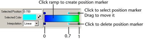
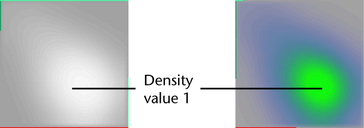
For example, suppose the Color Input is Density, and the color ramp ranges from blue on the far left to green on the far right.
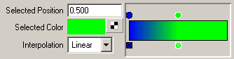
In a 2D container with Density values ranging from 0 to 1, the color of the Density would range from blue to green.
Advanced ramp features exist. See Advanced ramp features for more information.
Interpolation
Controls the way colors blend between positions on the ramp. The default setting is Linear.
Color Input
Defines the attribute used to map the color value.
The other options all set the Color Input to the color corresponding with the value from the grid. For example if Density is the Color Input, the color at the start of the color ramp is used for Density values of 0 and the color at the end of the ramp for Density values of 1.0. Midrange values map according to the Input Bias.
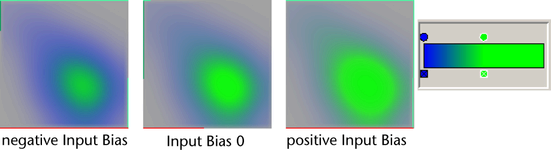
Color Input Bias adjusts the sensitivity of the selected Color Input. Input values of 0 and 1 always map to the start and end of the ramp, while the bias determines where in the ramp a value of 0.5 maps. If the Input Bias is 0.0 then a Color Input value of 0.5 maps to the exact middle of the color ramp. Instead of values that are very close using the color at one part of the ramp, you can use the full range of colors to represent the values.
For example, if Density is the Color Input and the Density values in the container are all close to 0.1, you can use the Input Bias to shift the ramp color range so the Density values around 0.1 can be differentiated using the full range of colors on the ramp. If you do not change the Input Bias, the differences in color for values close to 0.1 could be indistinguishable.
Incandescence controls the amount and color of light emitted from regions of Density due to self illumination. The particular colors selected from this range correspond with the values for the selected Incandescence Input. Incandescent emission is not affected by illumination or shadowing.
The Incandescence ramp defines a range of incandescent color values. The particular colors selected from this range correspond with the values for the selected Incandescence Input. Incandescence Input values of 0 map to the color at the left of the ramp, Incandescence Input values of 1 map to the color at the right of the ramp, and values between 0 and 1 map to the color corresponding with the position on the ramp (relative to the Input Bias).
You define the colors on the ramp by adding position markers to the ramp and changing the color at the markers.
Advanced ramp features exist. See Advanced ramp features for more information.
Interpolation
Controls the way colors blend between positions on the ramp. The default setting is Linear.
Incandescence Input
Defines the attribute used to map the incandescence color value.
The other options all set the Incandescence Input to the color corresponding with the value from the grid. For example if Temperature is the Incandescence Input, the color at the start of the incandescence ramp is used for Temperature values of 0 and the color at the end of the ramp for Temperature values of 1.0. Midrange values map according to the Input Bias.
Incandescence Input Bias adjusts the sensitivity of the selected Incandescence Input. Input values of 0 and 1 always map to the start and end of the ramp, while the bias determines where in the ramp a value of 0.5 maps. If the Input Bias is 0.0 then an Incandescence Input value of 0.5 maps to the exact middle of the color ramp. Instead of values that are very close using the color at one part of the ramp, you can use the full range of colors to represent the values.
For example, if Temperature is the Temperature Input and the Temperature values in the container are all close to 0.1, you can use the Input Bias to shift the ramp color range so the Temperature values around 0.1 can be differentiated using the full range of colors on the ramp. If you do not change the Input Bias, the differences in color for values close to 0.1 could be indistinguishable.
Opacity represents how much the fluid blocks light. The Opacity curve defines a range of opacity values used to render the fluid. The particular opacity values selected from this range are determined by the selected Opacity Input.
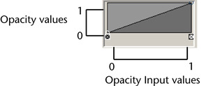
The vertical component represents the Opacity values from 0 (totally transparent) to 1 (totally opaque), the horizontal component represents Opacity Input values from 0 to 1. By clicking on the graph and dragging the points, you make a curve that defines what the opacity is for any input value. The default is a linear 1-1 relationship—input values (for example, Density) of 0 have no opacity, values of 0.5 have an opacity of 0.5, values of 1 have an opacity of 1.
Density is the default Opacity Input, and the default linear curve makes the Opacity exactly equal to the Density. Given that you cannot get more opaque than 1.0, Densities greater than 1.0 are totally opaque. This simulates the total saturation of a fluid (that is, so much smoke you have a block of solid carbon).
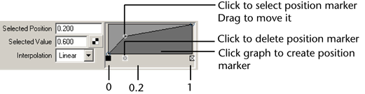
To give Density hard edges, like the edges on thick clouds, you can edit the Opacity curve to threshold out the thin Density (low Density values) and define a hard falloff. If you are dealing with very thin Density, positioning the markers on the curve for the desired falloff might involve the markers being very close together all the way to one edge of the curve. The Input Bias attribute allows you to define the general look of the function with an easy-to-read layout (that is, without crowding the values), and then affect the input range to map it to the desired part of the function.
Texturing is also applied to the inputs to opacity rather than the output. This allows you to use the Opacity curve to apply hard edges to the texture, rather than texturing a hard edged Density. The gain on the texture is simply how the texture affects opacity—small gain, small effect.
You could adjust the opacity of a fluid by moving the Transparency slider, ignoring all the other controls.
Interpolation
Controls the way values blend between position markers on the curve. The default setting is Linear.
The other options all set the Opacity Input value to the corresponding opacity value on the curve. For example if Density is the Opacity Input, the opacity value at the start of the curve is used for Density values of 0 and the opacity value at the end of the curve is used for Density values of 1.0. Midrange values map according to the Input Bias.
Opacity Input Bias adjusts the sensitivity of the selected Opacity Input used.
Input values of 0 and 1 always map to the start and end of the opacity curve, although the bias determines where in the curve a value of 0.5 maps. For example if you used Density as an input, and you want the fluid to become opaque at a Density of 0.001, then the Density bias can be used to shift most of the curve into this Density range. Instead of cramming several values at the beginning of the ramp you can use the full range. If the Input Bias is 0.0 then a value of 0.5 maps to the exact middle of the Opacity curve.
The attributes in this section control how this fluid shows up in the matte (alpha channel or mask) when you render with one. This is useful if you will be compositing your rendered images.
Matte Opacity Mode
Select how Maya uses the Matte Opacity value.
The Matte Opacity value is ignored, and all the matte for this fluid is set to be transparent. Use this option when you use substitute geometry in a scene to stand in for objects in a background image that you will be compositing with later. Your stand-in objects will ‘punch a hole’ in the matte. This allows other computer-generated geometry to pass behind your stand-in objects. Later, when foreground and background are composited, the results will be correct, with the background object showing through the ‘black hole’ areas.
The entire matte for the fluid is set to the value of the Matte Opacity attribute. This option is like Opacity Gain, except that the normally-calculated matte values are ignored in favor of the Matte Opacity setting. If there are transparent areas on the object, the transparency in these areas is ignored in the matte. Use this setting to composite an object with transparent areas, when you don’t want the background to show through them.
Matte Opacity has a default value of one, so by default Solid Matte and Opacity Gain have no effect.
(Not available on fluid texture.) Increase this value to increase the number of samples per ray used in the render, thereby increasing the shading quality of the render.
By mapping a texture to this attribute, you could define exactly which regions of a fluid got the highest shading quality (although the slowdown due to texturing might negate any benefits).
(Not available on fluid texture.) Defines the maximum contrast in the effective transparency of a volume span allowed by the Adaptive subdivisions sample method. When the contrast between two spans is greater than this value Maya subdivides the span. The contrast is defined as the effective difference in accumulated transparency from the viewpoint.
If this value is high, then the sampling will look like Uniform sampling.
If the Contrast Tolerance is low then the quality improves and the render time increases, although you will not require as many samples as uniform sampling for a given render quality.
The Quality setting should be just high enough that you do not miss dense regions altogether (this creates artifacts like dotty fringes around clouds).
Select the interpolation algorithm to use when retrieving values from fractional points within a fluid voxel when shading a ray. Sharply contrasting densities may show grid artifacts (like a mesh with no normal smoothing) with Linear interpolation. Smooth interpolation renders slower, but eliminates these problems.
Using the textures that are built into the fluidShape node you can increase the sampling time for high quality rendering. The sampling for the built-in textures is adaptive.
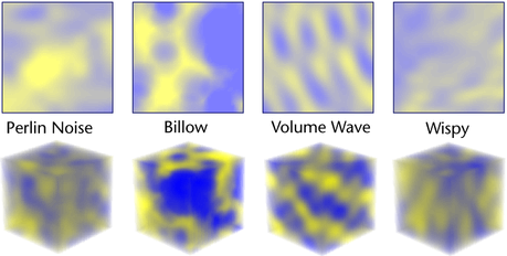
Texture Type
Select how to texture the Density in the container. The texture center is the center of the fluid.
Scales how fast coordinates are moved by Velocity when the Coordinate Method is Grid.
When Coordinate Speed is 1.0 the coordinates move through the volume at the same speed as the other properties (for example, Density). However this tends to result in the texture smearing out after a few steps.
Lower values tend to preserve the character of the texture and can look more natural.
Animating this value can be useful in some situations, such as when you do not want the texture to deform before a certain point (keyframe it to zero until the desired start point).
A scaling factor applied to all the values in the texture, centered around the texture’s average value. When you increase Amplitude, the light areas get lighter and the dark areas get darker.
If you set Amplitude to a value greater than 1.0, then those parts of the texture that scale out of range are clipped.
Controls how much calculation is done by the texture. Since the Fractal texture process produces a more detailed fractal, it takes longer to perform. By default, the texture chooses an appropriate level for the volume being rendered. Use Depth Max to control the maximum amount of calculation for the texture.
Use this attribute to animate the texture. You can keyframe the Texture Time attribute to control the rate and amount of change of the texture.
Type the expression "= time" into the edit cell to cause the texture to billow when rendered in an animation. Type "= time * 2" to make it billow twice as fast.
The zero point for the noise. Changing this value moves the noise through space.
The origin is relative to the noise Frequency. So if the noise is really stretched out in Y (larger Y-scale) the same offset will move it more in Y than the other directions. An advantage to this is that the noise loops when you offset the origin by 1.0.
Warps the noise function in a concentric fashion about a point defined by the Implode Center. When the Implode value is zero there is no effect. When the value is 1.0 it is a spherical projection of the noise function, creating a starburst effect. Negative values can be used to skew the noise outward instead of inward.
Controls how the cells for the Billow noise type are arranged relative to one another. Set Randomness to 1.0 to get a realistic random distribution of cells, as would be found in nature. If you set Randomness to 0, all the spots are laid out in a completely regular pattern. This can provide interesting effects when used as a bump map.
(Not available on fluid texture.)
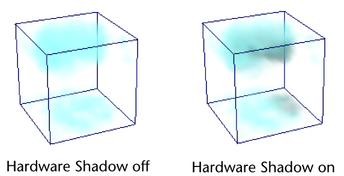
Use this attribute to brighten-up or darken shadows cast from the fluid.
When Shadow Opacity is 0.5, the shadows are attenuated in exact proportion to the transparency of the fluid.
When Shadow Opacity is zero, no shadowing occurs.
When Shadow Opacity is 1.0, shadows are completely black and the fluid is totally in shadow.
Values less than 0.5 can help make thick clouds appear more translucent.
Values greater than 0.5 make the clouds unnaturally opaque to lights, but may be useful to accentuate self shadowing.
Turn Real Lights on to use the lights in your scene.
Turn off Real Lights ignore the lights in the scene and instead use a single built-in directional light. The simple built-in lighting is faster, especially for self shadowing. It does not cast shadows or light onto other objects. Fluids using the built-in light do not receive shadows from other objects.