Most of the nodes in the Math category are fairly straightforward. Almost all of them support most of the data types, such as scalars and 3D vectors (but not colors — see Working with Colors in ICE). However, a few of the Math nodes deserve special mention.
The Multiply node can be used to multiply various data types. It accepts multiple inputs but they must be the same data type, and the output is always a value of the same data type as the inputs. For example, the product of two or more integers is an integer, the product of scalars is a scalar, and so on.
You can also use the Multiply node to n-dimensional multiply vectors together. In this case, the multiplication is component-wise, which can be useful for scaling non-uniformly. There are separate nodes for Dot Product and Cross Product.
Controlling Amplitude with Multiply by Scalar
The Multiply by Scalar node is very useful. You can use it anywhere you need an amplitude-like slider. Multiply by Scalar can be used to multiply almost any type of data, including scalars and 3D vectors.

Multiplying Vectors by Matrices
The Multiply Vector by Matrix node lets you multiply an n-dimensional vector by an n-by-n matrix in the usual way. The multiplication is performed as if the vector is a row-vector on the left and the matrix is on the right.
You can also use the Multiply Vector by Matrix node to multiply a 3D vector by a 4-by-4 matrix or a 4D vector by a 3-by-3 matrix. In these cases, special multiplication rules are used that assume homogeneous coordinates. See Using Geometry Queries.
The Random Value and Turbulence nodes can be used to generate randomized variations in values.
The Random Value node generates a pseudo-random value based on a mean value, a variance, and a distribution type. It can generate values of different data types such as scalar, vector, matrix, and so on. See Random Value [ICE Reference] for more information.
The generated sequence of numbers depends on three things:
Seed. If you require that two Random Value nodes generate different sets of random values, simply assign them different seed values.
ID. If you require that different particles get assigned different values, use a Get Data node to get the particles' ID and plug it into the ID port. For other types of components, you can plug their indices into the ID port — see Working with IDs and Indices.
Time Varying. If this is true, a different value will be generated every frame.
You can plug other attributes into the ID port if you want. For example, if you plug particles' Age into the ID port (a Round node will automatically be added to convert from scalar to integer), then all particles with the same age are assigned the same value.
In addition to the Random Value node, there are a number of compounds especially designed for randomizing in different ways or for randomizing specific things. For example, the Randomize Vector by Cone distributes vectors evenly in a cone or sphere shape instead of a box distribution, and the Randomize Value by Range lets you specify minimum and maximum values instead of a mean and variance. You can find all the various randomizing compounds by typing "rand" in the Quick Filter box of the preset manager.
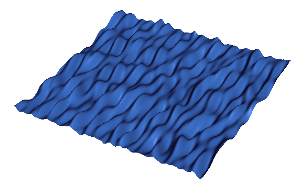
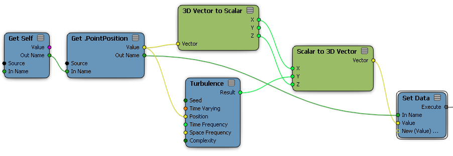
The Turbulence node creates a coherent noise pattern that varies continuously in space, as well as optionally in time. Instead of using ID to generate individual values, you use element positions. Values range between 1.0 and –1.0.

|
This illustration shows the turbulent noise pattern. The Turbulence node is used to set the point positions in Y. Space Frequency was set differently in X and Z, resulting in long, thin ripples. |

|
|
In addition to the Turbulence node, there are several Turbulize compounds designed to work with specific situations. You can find them all by typing "turb" in the quick filter box of the preset manager.
The FCurve node lets you use a profile curve to output a value (Y axis) based on an input (X axis). The X axis does not necessarily correspond to the current frame or time, unless you drive the input port with a Current Frame or Current Time node.
To expose the fcurve control in a compound, expand the Fcurve node fully and drag the Expose Input icon onto the Profile parameter.
The nodes in the Math/Statistics subcategory work on an entire data set, rather than individual values in a data set. For example, you can get the average Age of particles in a set.
Most of the Statistics nodes change context from per component to per object
There are two variations of the arctangent function in the Math/Trigonometry subcategory:
ArcTan accepts a single input and returns a result in the range (–90, 90).
ArcTan 2 accepts two inputs, X and Y, and calculates the arctangent of Y/X. It returns a result in the range (-180, 180). It uses the signs of X and Y to return a result in the corresponding quadrant, so for example, X = 1 and Y = 1 returns 45 degrees but X = –1 and Y = –1 returns –135 degrees.