The fundamental requirement of HI Solver is that the solution be history-independent: the solution has to be based on the goal and other incidental parameters solely at their current states.
Swivel Angle Degree of Freedom
When the positional goal is given for a single chain, there remains an obvious degree of freedom: the rotation about the End Effector Axis (EE Axis). The swivel angle is used to describe this degree of freedom quantitatively.
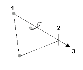
1. Start joint
2. End effector
3. EE axis
Let’s call the plane passing all the joints the Solver Plane. When joints do not lie on a plane, we will define it to be the plane that (A) passes the Start Joint and End Joint and (B) is closest to the remaining joint in a certain sense.
The Swivel Angle describes the degree of freedom of the Solver Plane and it constrains only the Start Joint.
In order to describe the solver plane in terms of a numerical quantity, we have to agree to what 0 means. Given the end-effector position, where is the Zero (Solver) Plane? The Zero Plane Map takes as the argument EE Axis and produces the normal to the zero plane.
The IK system allows individual solver plug-ins to define their own Zero Plane Maps. When not defined, the IK system provides a default one.
The argument to the Zero Plane Map is a unit vector to give the direction of the EE axis. Equivalently, when the EE slides along the EE axis, the solver plane should be fixed. Therefore, the Zero Plane Map defines a vector field on a sphere. Given a point on the sphere, it produces a tangential unit vector to be interpreted as the normal to the zero plane.
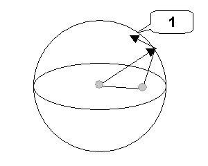
1. Normal to the zero plane
It is a mathematical fact that there does not exist a continuous vector field on a sphere. No matter how hard you try, there will always be a point on the sphere where neighboring vectors change dramatically. This is where the solver plane will flip when the end effector axis approaches to it.
This is because, on one hand, the history independent requirement demands us to assign a fixed vector to the singular point. On the other hand, no matter what vector is assigned, it will be dramatically different from some vectors assigned to the neighboring points.
Intrinsic Reference Frame for the Sphere
In order to define the Zero Plane Map, we need to define a reference frame for the sphere. This reference frame is intrinsic to the joint chain itself.
A sphere can be defined by the center, the horizontal plane, and the meridian (zero longitude). The center is assigned to the start joint.
The pose when all the joint angles assume preferred angles is particularly important. Let’s call it the preferred pose.
We use the solver plane at the preferred pose as the horizontal plane. Since the swivel angle is used to control the start joint, the preferred angles at the start joint are not so intrinsic. It is also reasonable to define the horizontal plane with the solver plane that is derived by assigning zeroes to the start joint and preferred angles to the other joints.
The EE axis defines the meridian. The sphere is now defined as shown in the following figure:
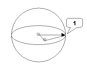
1. EE axis
All the joints assume preferred angles. The Zero Plane Map is to be defined on this sphere.
The API for the plug-in solver to define its own Zero Plane Map in fact takes the EE axis and the normal to the solver plane at the preferred pose:
virtual const IKSys::ZeroPlaneMap*

 GetZeroPlaneMap(const Point3& a0,
 const Point3& n0) const
where a0 and n0 are the EE axis and solver plane at the preferred pose, respectively. Object of ZeroPlaneMap is a function that assigns a plane normal to each point on the sphere.
When not provided by plug-in solvers, (the IK Solver itself is implemented as a plug-in solver) the IK system will provide a default one. This map is defined by the following rules:
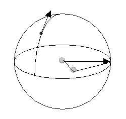
Deriving the default normal to the zero plane
Obviously, this method won’t extend to the north or south poles. They are the singular points. When the EE axis moves across the poles, the normal will suddenly change direction: it flips from the users’ viewpoint.
Normally, the preferred pose is the one when the solver is first assigned. So, the plane on which one lays the joints corresponds to the horizontal plane here. Rule A makes sure that the chain will stay on the plane if one moves the goal on the plane.
Rule B means that, when you move the goal along the great circle vertical to the equator, the chain will stay vertical, except when it passes through the poles, which are the singular points of this map.
So far, we have described things as if the whole world comprises only IK elements. In practice, the IK chain and goal might sit at points of separate transformation hierarchies. Ultimately, we need to map the position of the end effector that is described in the world to a point on the sphere. Depending how the sphere is mounted relative to the end effector position, the readings of latitude and longitude are different. The parent transformation space that this sphere is to be placed in is called the Swivel Angle Parent Space, or Parent Space when the context is clear.
The parent space has to be invariant with regard to the IK parameters. Right now, we provide two choices:
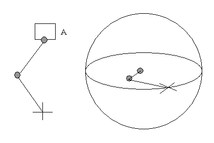
If both the start joint and the goal are rooted directly at the world, the choice of Parent Space does not give rise to any difference. In the following example, the start joint is parented to object A.

The IK chain is parented (via the start joint) at object A.
Assume this is the pose when the IK solver is assigned. So, this is the preferred pose. The plane on that the joints are laid out is the horizontal plane of the (Zero Plane Map) sphere.
In the following example, we look at a case where there exists a rotation in the parent space when the IK solver is assigned.
The parent space of the IK chain contains a rotation when the IK solver is assigned.
Parent A contains a rotation of 90 degrees. This is an abstraction of the case when a user creates four bones without an IK solver and later assigns an IK solver from Bone2 to Bone4. If we parent the chain directly to world, it would appear as shown in the right figure: the solver plane becomes horizontal.
A problem of B is that the figure on the right is never shown to the user. They have to envision it in order to understand the flipping.
This example describes what happened when Start Joint is reassigned. Suppose we have an IK chain of four bone nodes.
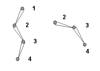
1. Bone01
2. Bone02
3. Bone03
4. Bone04
The Start and End Joints are Bone01 and Bone04, respectively. Suppose the pose shown in the figure is the preferred pose and Bone01 contains a rotation. If we parent Bone02 directly to the world, the hierarchy from Bone02 will appear as in the right figure.
When we reassign Start Joint to Bone02, the Zero Plane Map sphere will be based on the configuration on the right.
If you delete the solver/goal and assigned a new one from Bone02 to Bone04, you will find that the chain won’t flip. Why? Assignment of Start Joint is different from creating a new IK chain/goal. Start Joint is one of many IK parameters. Reassigning it is simply the same as modifying any parameter. The rest parameters are intact. In particular, the Swivel Angle is not changed as a result of this reassignment.
Creating a new IK chain/goal is different. Effort is made to ensure that the joint chain stay fixed by adjusting parameters appropriately. In particular, the Swivel Angle will be set to a value so that the solver plane keeps stationary in the viewport.


