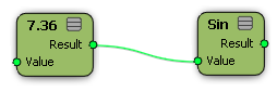
In general, you connect ICE nodes by clicking and dragging an output port from the right of one node onto another node and then selecting an input port. You can also connect two nodes by dragging the other way, from an input port onto an output port. Data flows along the connection from the output port to the input port and gets processed by the next node in the chain.
When a port is connected, the value of the corresponding parameter is driven by the connection. You can no longer set the parameter's value in the node's property editor. In addition, its controls (checkboxes, sliders, etc.) are not displayed. If you remove the connection, the controls reappear in the property editor.
There are some special factors that determine whether you can connect two specific ports:
The type of the data, as indicated by the port colors. See Data Types.
The context of the data. See Context.
The structure of the data. See Structure.
If you cannot connect two ports, it is likely because one or more of these things are incompatible.
Some nodes have a fixed number of input ports, such as Divide by Scalar. However, other nodes allow an arbitrary number of connections. For example, Multiply allows any number of values to be multiplied together. See Managing Multiple Ports.
Nodes can be displayed in three possible states:
Expanded: Shows all output and input ports. This is useful when you are actively making and adjusting connections on a node.
Collapsed: Shows no ports. This can be useful when you are finished with a portion of a tree and want to simplify the view.
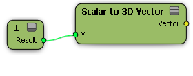
Show Connections Only: This is a partially expanded and partially collapsed state that shows all output ports and all connected input ports. This can be useful when you are done making input connections but still want to see how they are connected.
When a connected port is hidden, you can display information about it by hovering the mouse pointer over the connecting line.
On some nodes, the input ports are organized into port layout groups. These are represented by triangles and bold text. When a node is expanded, you can collapse and expand these layout groups individually by clicking on the triangle.
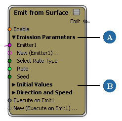
Port layout groups shown as expanded (A) and as collapsed (B).
If a node already exists in the tree, you can connect one of its output ports by dragging the port icon onto another node. Alternatively for base nodes (not compounds), you can also add a new node and connect it at the same time by dragging the node from the preset manager onto a port or connection.
Click on an output port on the right of a node, then drag it over another node. As you drag, you should see an arrow representing the connection. Dragging a connection to the edge of the workspace automatically scrolls the view.
If the list of ports is not completely expanded (that is, not all input ports are visible), release the mouse button and a popup menu appears showing all input ports that are valid for that connection. Select an item from the menu to connect to that port. Ports that are already driven by a connection are displayed with a bullet in the menu; selecting a port that is already connected replaces the old connection with the new one. You can press Shift to keep the menu open while you select multiple ports.
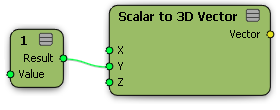
If the list of ports is completely expanded, release the mouse button over a specific input port to connect. Valid ports are highlighted in white when the mouse pointer moves over them.
You can connect the same output to as many inputs as you want.
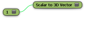
Drag a base node (not a compound) from the preset manager onto the node you want to connect to. The new node's outline should display an arrow instead of a plus sign when you release the mouse button.
If the desired input port is displayed, drag the new node over it. When the port is highlighted, release the mouse button.
If the desired input port is not displayed, simply release the mouse button over the node, making sure that you don't accidentally highlight an unwanted port before you release. If there is only one valid input port, it will be connected automatically. Otherwise, select the desired port from the menu that pops up. Ports that are already connected are shown with a bullet, but you can still select them to replace the existing connection.
Drag a base node (not a compound) from the preset manager onto the line that represents a connection. Release the mouse button when the curve is partially highlighted and the new node's outline shows an arrow instead of a plus sign.
The new nodes inputs and outputs are connected according to the first valid ports available. If these are not the desired ports, simply reconnect them.
Inserting nodes in this manner is useful in many situations, such as adding a Multiply by Scalar node for increased control over an amplitude.
Move the mouse pointer over the line near the connection to the input port. The line is highlighted in white.
Click and drag away from the port until the pointer changes to a pair of scissors, and then release the mouse button.
You can also replace a connection by connecting a new node without disconnecting the first one.
The data type defines the kind of values that a port can pass or accept, such as Boolean, integer, scalar or vector.
You cannot connect two ports if their data types are incompatible. However, you can convert between many data types using the nodes in the Conversion category (Tools). In some cases, conversion nodes are added automatically when you try to connect ports; for example, a Round node is inserted when you connect a scalar output into an integer input.
The different port types and their associated data types are summarized in the table below.
| Type |
Description |
|
|---|---|---|

|
Polymorphic |
Accepts a variety of data types. See Polymorphic Ports. |

|
Boolean |
A Boolean value: True or False. |

|
Integer |
A positive or negative number without decimal fractions, for example, 7, –2, or 0. |

|
Scalar |
A real number represented as a decimal value, for example, 3.14. Internally this is a single-precision float value. |

|
Color |
A color value expressed as a quadruple of scalars representing the RGBA channels. |

|
2D Vector |
A two-dimensional vector [x, y] whose entries are scalars, for example, a UV coordinate. |

|
3D Vector |
A three-dimensional vector [x, y, z] whose entries are scalars, for example, a position, velocity, or force. |

|
4D Vector |
A four-dimensional vector [w, x, y, z] whose entries are scalars. |

|
Quaternion |
A quaternion [x, y, z, w]. Quaternions are usually used to represent an orientation. Quaternions can be easily blended and interpolated, and help address gimbal-lock problems when dealing with animated rotations. |
|
|
Rotation |
A rotation as represented by an axis vector [x, y, z] and an angle in degrees. |

|
3x3 Matrix |
A 3-by-3 matrix whose entries are real numbers. 3x3 matrices are often used to represent rotation and scaling. |

|
4x4 Matrix |
A 4-by-4 matrix whose entries are real numbers. 4x4 matrices are often used to represent transformations (scaling, rotation, and translation). |

|
Shape |
A primitive geometrical shape, or a reference to the shape of an object in the scene. This data type is used to determine the shape of particles. |

|
Geometry |
A reference to a geometrical object in the scene, such as a a polygon mesh, NURBS curve, NURBS surface, or point cloud. You can sample the surface of a geometry to generate surface locations for emitting particles. |

|
Surface Location |
A location on the surface of a geometric object. The locator is "glued" to the surface of the object so that even if the object transforms and deforms, the locator moves with the object and stays in same relative position. |

|
String |
A string of characters. Strings can be used by custom nodes for storing file paths, for example. |

|
Topology |
The topology of a polygon mesh object. This is used in ICE modeling. |

|
Execution |
Not a data type in the conventional sense. You connect Execution ports such as the output of a Set Data into an Execute or root node to control the flow of execution in the tree. |
|
|
Reference |
Also not a data type in the conventional sense. This is a reference to an object, parameter, or attribute in the scene, expressed as a character string. You can daisy-chain these as described in Daisy-chaining References. |
Polymorphic ports can accept several different data types. For example, the Add node can be used to add together two or more integers, or two or more scalars, or two or more vectors, and so on.
Once you connect a value to a polymorphic port, its port type becomes resolved. Other input and output ports on the same node and on connected nodes may also become resolved and only accept specific data types. This reflects the fact that, for example, you cannot add an integer to a vector.
|
|
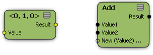
| Before anything is connected, the Add node's ports are unresolved (black). |
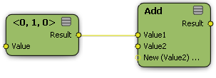
Once a node is connected to Value1, then Value2 and Result become resolved. In this case, they are yellow for 3D vectors. |
Even after a port's type has been resolved, you can still change it by replacing the connection with a different data type. However, this works only if the port is not resolved by other connections in the tree.
Note that a port's color doesn't change back when the data type is no longer forced by connected nodes. This indicates that the data type is still resolved, although it can be changed by connecting something else so in a sense it's still polymorphic. This can also true of compounds that you add to a tree, where a port's color may suggest that it accepts only certain connections when you can actually connect anything.
If a port's type is unresolved, you cannot set values in its property editor. Once it is resolved, the appropriate controls appear in the property editor. Different data types use different controls: for example, checkboxes for Booleans, sliders for scalars, and so on.
|
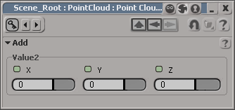
|
| Before any connection, the Add node's property editor is blank. |
After connection, controls appear for Value2. There are no controls for Value1 because it is being driven by the connection. |
While polymorphic ports accept several data types, they don't necessarily accept all types of connection. For example, the ports of a Pass Through node accept any type of value, but it doesn't make sense to use a Multiply by Scalar node with a Boolean value.
For two ports to be connectable, their contexts must be compatible. The context is essentially the owner of the data: the object itself, or its points, polygons, edges, polynodes, etc. For example, if there's one value for the whole object then you cannot set a new value per point. On the other hand, if the context is per point then each point has its own value, and setting the value for one point does not affect the other points' values.
Context is determined by two factors:
The data context gets propagated through node connections in the same way as the data types of polymorphic nodes.
The context of data in the tree is partly determined by the type of element that it is associated with: point, edge, polygon, object, etc. For example, you can't add point positions to polygon normals. Both values are 3D vectors, but there are fewer polygons than points in a typical mesh and there is no natural way to determine which point position to add to which polygon normal — in other words, they belong to different contexts.
The following table shows the different types of element that define contexts:
| Context |
Description |
|---|---|
| Singleton |
A data set containing exactly one value. For example, an object's position, a bone's length, a mesh's volume, etc. For more information, see Singleton Context. |
| Point |
A data set containing one value for each point of a geometric object (point cloud, polygon mesh, NURBS surface, curve, lattice, etc.). For example, point positions, envelope weight assignments, etc. |
| Line |
A data set containing one value for each edge, subcurve, or surface boundary. For example, edge lengths. |
| Face |
A data set containing one value for each polygon or subsurface. For example, polygon normals or polygon areas. |
| Sample |
A data set containing one value for each texture sample of a geometry. A sample is usually a polygon node on a polygon mesh, but there can also be samples on NURBS surfaces and curves. |
Just as the type of component data determines the context, so does the object that the components belong to. For example, you can't add the point positions of one object to the point positions of another object. There is no natural way to determine which specific pairs of point positions get added, and in general the two objects may not even have the same number of points. There is one exception — when objects are duplicates — and in this case you can use the Switch Context node as described in Switching Contexts.
Data that belongs to an object, instead of an object's components, is different. In most cases this data belongs to the singleton context, described next.
Data sets containing exactly one value belong to the singleton context. Singleton data is always compatible with other singleton data, no matter which object it is associated with.
Singleton data is also usually compatible with other data contexts. For example, you can add an object's position (singleton context) to its point positions (point context). You can even add an object's position to a different object's point positions.
There are cases where data sets are not bound to elements on an object in the scene. For example, the Generate Sample Set node generates a set of random point locators on the surface of a geometric object. In the following tree, a point is added to the point cloud at each point locator.
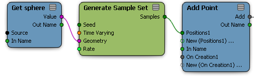
The size of the set of point locators passed from the Generate Sample Set node to the Add Point node does not necessarily match the number of any kind of element in the scene. This size of the set is actually controlled by the rate parameter of the Generate Sample Set node. In such a case, the context of this data is owned by the Generate Sample Set node.
Node-bound contexts are typically incompatible with each other. For example, if you generate two sets of locations on the same geometry, they are bound to different nodes and cannot be combined.
In addition to data type and context, structure is another thing that determines the compatibility of ports. There are two structures: single and array (ordered set).
The single structure has one value for each element of a data set. For example, each point position is a single 3D vector.
The array structure has zero, one, or more values for each member of a data set. The number of values in the array can be different for different members of the data set. For example, the neighbors of points on a polygon mesh would be arrays with a different number of values depending on each point's connectivity.
For more information about working with arrays, see Working with Arrays in ICE Trees.
 Except where otherwise noted, this work is licensed under a Creative Commons Attribution-NonCommercial-ShareAlike 3.0 Unported License