Overview

This guide describes the Maya features for accelerating playback and manipulation of animated scenes. It covers key concepts, shares best practices/usage tips, and lists known limitations that we aim to address in subsequent versions of Maya.

This guide will be of interest to riggers, TDs, and plug-in authors wishing to take advantage of speed enhancements in Maya.

If you would like an overview of related topics prior to reading this document, check out Supercharged Animation Performance in Maya 2016.

Key Concepts

Starting from Maya 2016, Maya accelerates existing scenes by taking better advantage of your hardware. Unlike previous versions of Maya, which were limited to node-level parallelism, Maya now includes a mechanism for scene-level analysis and parallelization. For example, if your scene contains different characters that are unconstrained to one another, Maya can evaluate each character at the same time.

Similarly, if your scene has a single complex character, it may be possible to evaluate rig sub-sections simultaneously. As you can imagine, the amount of parallelism depends on how your scene has been constructed. We will get back to this later. For now, let’s focus on understanding key Maya evaluation concepts.

At the heart of Maya’s new evaluation architecture is an Evaluation Manager (EM), responsible for handling the parallel-friendly representation of your scene. It maintains (and updates while the scene is edited) a few data structures (described below) used for efficient evaluation.

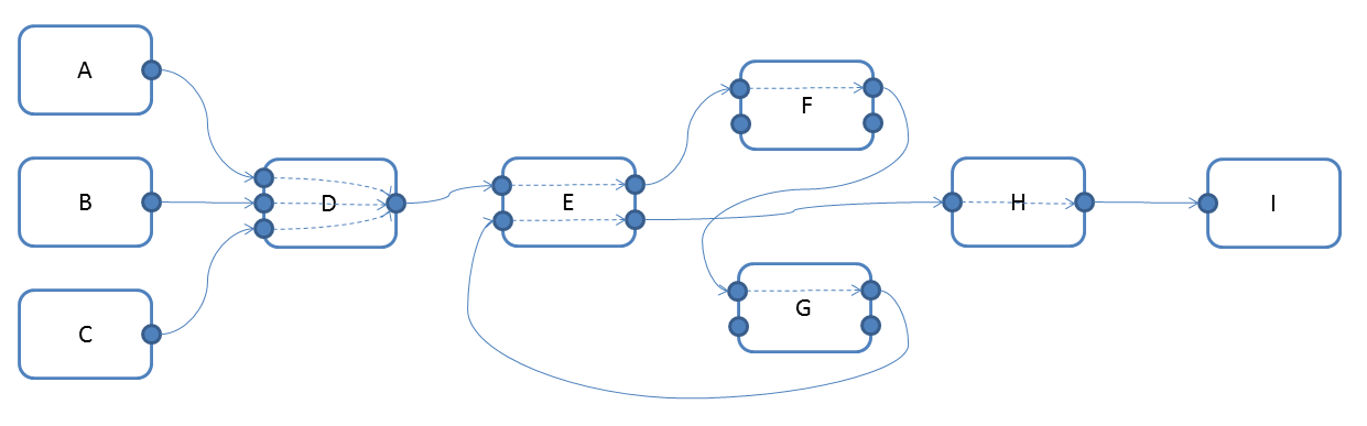
The basic description of the scene is the Dependency Graph (DG), consisting of DG nodes and connections. Nodes can have multiple attributes, and instances of these attributes on a specific node are called plugs. The DG connections are at the plug level, that is, two nodes can be connected to one another multiple ways through different plugs. Generally speaking, these connections represent data flow through the nodes as they evaluate. The following image shows an example DG:

The dotted arrows inside the nodes represent an implicit computation dependency between an output attribute (on the right of the node) and the input attributes (on the left) being read to compute the result stored in the output.

Before Parallel Maya, the DG was used to evaluate the scene using a Pull Model or Pull Evaluation. In this model, the data consumer (for instance the renderer) queries data from a given node. If the data is already evaluated, the consumer receives it directly. However, if the data is dirty, the node must first recompute it. It does so by pulling on the inputs required to compute the requested data. These inputs can also be dirty, in which case the evaluation request will then be forwarded to those dirty sources until it reaches the point where the data can be evaluated. The result then propagates back up in the graph, as the data is being “pulled”.

This evaluation model relies on the ability to mark node data as invalid and therefore requiring new evaluation. This mechanism is known as the Dirty Propagation in which the invalid data status propagates to all downstream dependencies. The two main cases where dirty propagation happened in the Pull Evaluation model were when:

• the current time is changed: in this case, animation curves no longer have the right value which depends on the current time. Therefore, dirty propagation starts from each animation curve and the dirty status is propagated through the graph to reach everything depending on time, directly or indirectly.
• a value is changed on a node: whether the value is being changed through interactive manipulation or by a script, all data that depends on this new value must be recomputed. Therefore, dirty propagation starts from the edited plug and the dirty status is propagated through the graph to reach everything depending on the edited attribute.

The Pull Evaluation model is not well suited for efficient parallel evaluation because of potential races that can arise from concurrent pull evaluations.

To have tighter control over evaluation, Maya now uses a Forward Evaluation model to enable concurrent evaluation of multiple nodes. The general idea is simple: if all a node’s dependencies have been evaluated before we evaluate the given node, pull evaluation will not be triggered when accessing evaluated node data, so evaluation remains contained in the node and is easier to run concurrently.

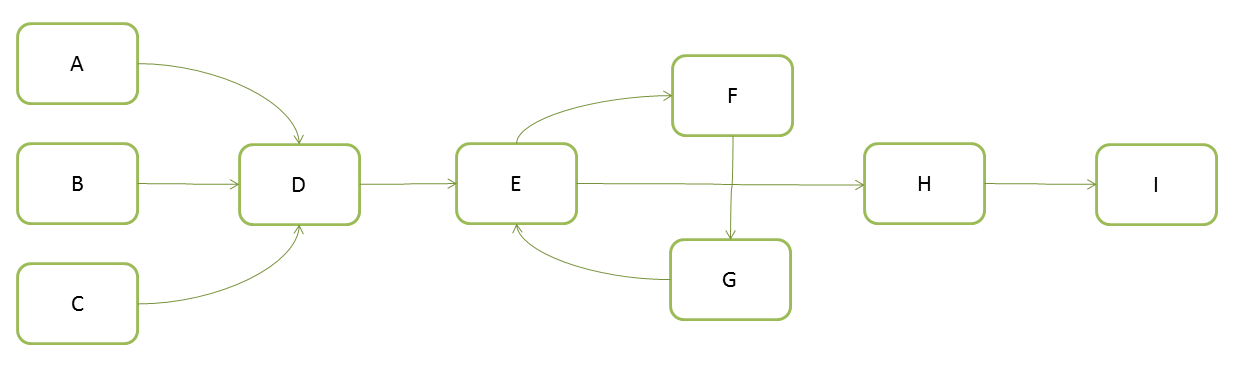
All data dependencies between the nodes must be known to apply this evaluation model, and this information is captured in the Evaluation Graph (EG), containing Evaluation Nodes. The EM uses dirty propagation to capture dependency information between the nodes, as well as which attributes are animated. EG connections represent node-level dependencies; destination nodes employ data from source nodes to correctly evaluate the scene. One important distinction between the DG and the EG is that the former uses plug-level connections, while the latter uses node-level connections. For example, the previous DG would create the following EG:

A valid EG may not exist or become invalid for various reasons. For example, you have loaded a new scene and no EG has been built yet, or you have changed your scene, invalidating a prior EG. However, once the EG is built, unlike previous versions of Maya that propagated dirty on every frame, Maya now disables dirty propagation, reusing the EG until it becomes invalid.

Tip. If your scene contains expression nodes that use getAttr, the DG graph will be missing explicit dependencies. This results in an incorrect EG. Expression nodes also reduce the amount of parallelism in your scenes (see Scheduling Types for details). Consider removing getAttr from expressions and/or using utility nodes.

While the EG holds the dependency information, it is not ready to be evaluated concurrently as-is. The EM must first create units of work that can be scheduled, that is, tasks. The main types of task created are:

• Individual Nodes: in the simplest case, an evaluation node can be computed directly. The task therefore consists of evaluating all of its animated attributes.
• Cycle Clusters: depending on the scene, the EG may contain circular node-level dependencies. If this is the case, the EM creates clusters that group together nodes in the same cycle. At scene evaluation time, nodes in cycle clusters are evaluated serially before continuing with other parallel parts of the EG, hence the evaluation of a cycle cluster consisting of a single task. While node-level cycles are perfectly legal, creating scenes with attribute-level cycles should be avoided as this is unsupported and leads to unspecified behavior.
• Custom Evaluator Clusters: the EM supports the concept of custom evaluators to override evaluation of sub-section of the EG. One example of this is the GPU override, which uses your graphics card’s graphics processing unit (GPU) to accelerate deformations. The custom evaluators will create clusters for nodes for which they take responsibility, and the EM creates a task for each of these clusters. At scene evaluation time, control is passed to the specific custom evaluator when the task is up to be executed.

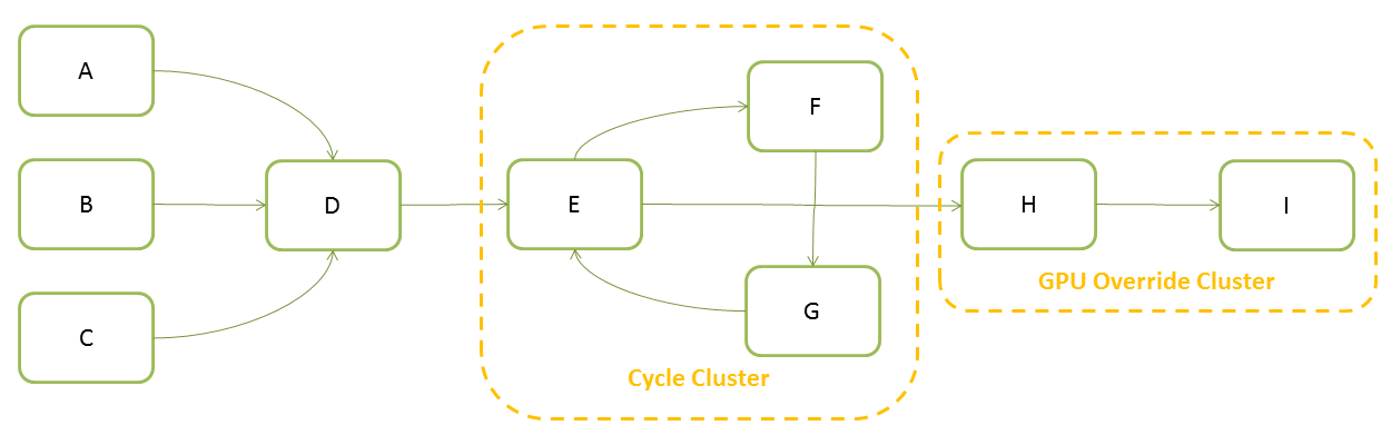
This step, called partitioning, is where the EM creates the individual pieces of work that will have to be executed. Each of these tasks will map to a Scheduling Node in the Scheduling Graph (SG), where connections represent dependencies between the tasks:

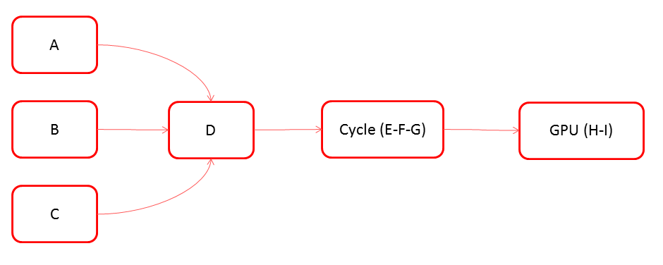
The SG is an acyclic graph, otherwise it would be impossible to schedule nodes in a cycle since there would be no starting point for which all dependencies could be evaluated. In addition to the dependencies that come directly from the EG, the SG can have additional scheduling constraints to prevent concurrent evaluation of subsets of nodes (see Scheduling Types for details).

Supported Evaluation Modes

Starting in Maya 2016, 3 evaluation modes are supported:

When using either Serial or Parallel EM modes, you can also activate GPU Override to accelerate deformations on your GPU. You must be in Viewport 2.0 to use this feature (see GPU Override).

To switch between different modes, go to the Preferences window (Windows > Settings/Preferences > Preferences > Animation). You can also use the evaluationManager MEL/Python command; see documentation for supported options.

To see the evaluation options that apply to your scene, turn on the Heads Up Display Evaluation options (Display > Heads Up Display > Evaluation).

First Make it Right Then Make it Fast

Before discussing how to make your Maya scene faster using Parallel evaluation, it is important to ensure that evaluation in DG and EM modes generates the same results. If you see different results in the viewport during animation (as compared to previous versions of Maya), or tests reveal numerical errors, it is critical to understand the cause of these errors. Errors may be due to an incorrect EG, threading related problems, or other issues.

Below, we review Evaluation Graph Correctness and Thread Safety, two important concepts to understand errors.

Evaluation Graph Correctness

If you see evaluation errors, first test your scene in Serial evaluation mode (see Supported Evaluation Modes). Serial evaluation mode uses the EM to build an EG of your scene, but limits evaluation to a single core to eliminate threading as the possible source of differences. Note that since Serial evaluation mode is provided for debugging, it has not been optimized for speed and scenes may run slower in Serial than in DG evaluation mode. This is expected.

If transitioning to Serial evaluation eliminates errors, this suggests that differences are most likely due to threading-related issues. However, if errors persist (even after transitioning to Serial evaluation) this suggests that the EG is incorrect for your scene. There are a few possible reasons for this:

Custom Plugins. If your scene uses custom plug-ins that rely on the mechanism provided by the MPxNode::setDependentsDirty function to manage attribute dirtying, this may be the source of problems. Plug-in authors sometimes use MPxNode::setDependentsDirty to avoid expensive calculations in MPxNode::compute by monitoring and/or altering dependencies and storing computed results for later re-use.

Since the EM relies on dirty propagation to create the EG, any custom plug-in logic that alters dependencies may interfere with the construction of a correct EG. Furthermore, since the EM evaluation does not propagate dirty messages, any custom caching or computation in MPxNode::setDependentsDirty is not called while the EM is evaluating.

If you suspect that your evaluation errors are related to custom plug-ins, temporarily remove the associated nodes from your scene and validate that both DG and Serial evaluation modes generate the same result. Once you have made sure this is the case, revisit the plug-in logic. The API Extensions section covers Maya SDK changes that will help you adapt plug-ins to Parallel evaluation.

Another debugging option is to use “scheduling type” overrides to force custom nodes to be scheduled more conservatively. This approach enables the use of Parallel evaluation even if only some of the nodes are thread-safe. Scheduling types are described in more detail in the Thread Safety section.

Errors in Autodesk Nodes. Although we have done our best to ensure that all out-of-the-box Autodesk Maya nodes correctly express dependencies, sometimes a scene uses nodes in an unexpected manner. If this is the case, we ask you make us aware of scenes where you encounter problems. We will do our best to address problems as quickly as possible.

Thread Safety

Prior to Maya 2016, evaluation was single-threaded and developers did not need to worry about making their code thread-safe. At each frame, evaluation was guaranteed to proceed serially and computation would finish for one node prior to moving onto another. This approach allowed for the caching of intermediate results in global memory and using external libraries without considering their ability to work correctly when called simultaneously from multiple threads.

These guarantees no longer apply. Developers working in recent versions of Maya must update plug-ins to ensure correct behavior during concurrent evaluation.

Two things to consider when updating plug-ins:

• Different instances of a node type should not share resources. Unmanaged shared resources can lead to evaluation errors since different nodes, of the same type, can have their compute() methods called at the same time.

• Avoid non thread-safe lazy evaluation. In the EM, evaluation is scheduled from predecessors to successors on a per-node basis. Once computation has been performed for predecessors, results are cached, and made available to successors via connections. Any attempt to perform non-thread safe lazy evaluation could return different answers to different successors or, depending on the nature of the bug, instabilities.

Here’s a concrete example for a simple node network consisting of 4 nodes:

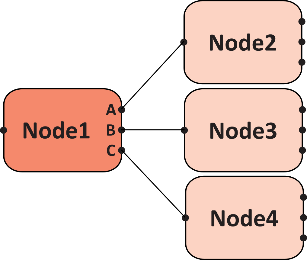
In this graph, evaluation first calculates outputs for Node1 (that is, Node1.A, Node1.B, Node1.C), followed by parallel evaluation of Nodes 2, 3, and 4 (that is, Read Node1.A to use in Node2, Read Node1.B to use in Node3, and so on).

Knowing that making legacy code thread-safe requires time, we have added new scheduling types to provide control over how the EM schedule nodes. Scheduling types provide a straightforward migration path, so you do not need to hold off on performance improvements, just because a few nodes still need work.

There are 4 scheduling types:

By default, nodes scheduled as Serial provide a middle ground between performance and stability/safety. In some cases, this is too permissive and nodes must be downgraded to GloballySerial or Untrusted. In other cases, some nodes can be promoted to Parallel. As you can imagine, the more parallelism supported by nodes in your graph, the higher level of concurrency you are likely to obtain.

Tip. When testing your plug-ins with Parallel Maya, a simple strategy is to schedule nodes with the most restrictive scheduling type (that is, Untrusted), and then validate that evaluation produces correct results. Raise individual nodes to the next scheduling level, and repeat the experiment.

There are three ways to alter the scheduling level of your nodes:

Evaluation Toolkit. Use this tool to query or change the scheduling type of different node types.

C++/Python API methods. Use the OpenMaya API to specify the desired node scheduling by overriding the MPxNode::schedulingType method. This function should return one of the enumerated values specified by MPxNode::schedulingType. See the Maya MPxNode class reference for more details.

MEL/Python Commands. Use the evaluationManager command to change the scheduling type of nodes at runtime. Below, we illustrate how you can change the scheduling of scene transform nodes:

The Evaluation Toolkit and MEL/Python Commands method to alter node scheduling level works using node type overrides. They add an override that applies to all nodes of a given type. Using C++/Python API methods and overriding the MPxNode::schedulingType function gives the flexibility to change the scheduling type for each node instance. For example, expression nodes are marked as globally serial if the expression outputs are a purely mathematical function of its inputs.

The expression engine is not thread-safe so only one expression can run at a time, but it can run in parallel with any other nodes. However, if the expression uses unsafe commands (expressions could use any command to access any part of the scene), the node is marked as untrusted because nothing can run while the expression is evaluated.

This changes the way scheduling types should be queried. Using the evaluationManager command with the above flags in query mode will return whether an override has been set on the node type, using either the Evaluation Toolkit or the MEL/Python commands.

The Evaluation Toolkit window lets you query both the override type on the node type (which cannot vary from one node of the same type to the other), or the actual scheduling type used for a node when building the scheduling graph (which can change from one node instance to the other).

Safe Mode

On rare occasions you may notice that Maya switches from Parallel to Serial evaluation during manipulation or playback. This is due to Safe Mode, which attempts to trap errors that possibly lead to instabilities. If Maya detects that multiple threads are attempting to simultaneously access a single node instance, evaluation will be forced to Serial execution to prevent problems.

Tip. If Safe Mode forces your scene into Serial mode, the EM may not produce the expected incorrect results when manipulating. In such cases you can either disable the EM:

cmds.evaluationManager(mode="off")

or disable EM-accelerated manipulation:

cmds.evaluationManager(man=0)

While Safe Mode exposes many problems, it cannot catch them all. Therefore, we have also developed a special Analysis Mode that performs a more thorough (and costly) check of your scene. Analysis mode is designed for riggers/TDs wishing to troubleshoot evaluation problems during rig creation. Avoid using Analysis Mode during animation since it will slow down your scene.

Evaluation Graph Invalidation

As previously described, the EG adds necessary node-level scheduling information to the DG. To make sure evaluation is correct, it’s critical the EG always be up-to-date, reflecting the state of the scene. The process of detecting things that have changed and rebuilding the EG is referred to as graph invalidation.

Different actions may invalidate the EG, including:

• Adding/removing nodes
• Changing the scenes transformation (DAG) hierarchy
• Adding/removing extension attributes
• Loading an empty scene or opening a new file

Other, less obvious, actions include:

• Static animation curves. Although animation curves are time-dependent, DG evaluation treats curves with identical (static) keys as time-independent to avoid unnecessary calculations. The EG uses a similar optimization, excluding and avoiding scheduling of static animation curves. This keeps the EG compact, making it fast to build, schedule, and evaluate. A downside of this approach is that changes to static animation curves will cause the EG to become invalid; on time change Maya will rebuild the EG and determine if curves should be treated as time-dependent and added to the EG.
• Dirty propagation crossing the Evaluation Graph. The DG architecture allowed for implicit dependencies (that is, dependencies not expressed via connections), using them during dirty propagation. When dirty propagation is detected for these implicit dependencies, the EG will invalidate itself since this could signal the need to add new dependencies to the EG.

Frequent graph invalidations may limit parallel evaluation performance gains or even slow it down (see Idle Actions), since Maya requires DG dirty propagation and evaluation to rebuild the EG. To avoid unwanted graph rebuilds, consider adding 2 keys, each with slightly different values, on rig attributes that you expect to use frequently. You can also lock static channels to prevent creation of static animation curves during keying. We expect to continue tuning this area of Maya, with the goal of making the general case as interactive as possible.

Tip. You can use the controller command to identify objects that are used as animation sources in your scene. If the Include controllers in evaluation graph option is set (see Windows > Settings/Preferences > Preferences, then Settings > Animation), the objects marked as controllers will automatically be added to the evaluation graph even if they are not animated yet. This allows Parallel evaluation for manipulation even if they have not yet been keyed.

Idle Actions

In this section, we discuss the different idle actions available in Maya that helps rebuild the EG without any intervention from the user. Prior to Maya 2019, only one idle action, the EG rebuild, was available, but it was not enabled by default. Since Maya 2019, we have added another idle action, the EG preparation for manipulation, and both of these are enabled by default.

Here is a description of the idle actions:

Tip. You can use the evaluationManager command to change which idle actions are enabled. You can enable and disable both idle actions individually.

Benefits

To make use of the Parallel Evaluation and GPU deformation during manipulation, the EG needs to be properly built, partitioned and scheduled, otherwise it will revert to DG. These idle actions allow the EG to automatically build and be ready to use when needed, since they are triggered at file load and after graph invalidation.

If you use Cached Playback, your cache automatically refills, too. This way, you can start playing from cache as soon as the scene is loaded or after you modify to the scene.

Caveats

In a typical frame evaluation, temporary values that are set on keyed attributes are restored to their original values, that is, the values on their associated curves. With the idle actions, this is an unwanted behavior, otherwise you would not be able to do any modifications to keyed attributes. To circumvent that issue, we had to add some special behaviougs One of these is the dirty propagation from stale plugs after an idle preparation for manipulation. When not in idle preparation for manipulation, this operation is done during the partitioning and scheduling phase. With idle preparation for manipulation, this operation is done at the next complete evaluation. Therefore, if you have many static curves, you might experience a slowdown on the first frame of playback.

If you do frequent operations that invalidate the graph or partitioning, you may experience some slowdowns due to the graph always being rebuilt. In such cases, it is advised that you disable the offending idle action until you are done.

Custom Evaluators

In this section, we describe mechanisms to perform targeted evaluation of node sub-graphs. This approach is used by Maya to accelerate deformations on the GPU and to catch evaluation errors for scenes with specific nodes. Maya 2017 also introduced new Open API extensions, allowing user-defined custom evaluators.

Tip. Use the evaluator command to query the available/active evaluators or modify currently active evaluators. Some evaluators support using the nodeType flag to filter out or include nodes of certain types. Query the info flag on the evaluator for more information on what it supports.

# Returns a list of all currently available evaluators.
import maya.cmds as cmds
cmds.evaluator( query=True )
# Result: [u'invisibility',
u'frozen',
...
u'transformFlattening',
u'pruneRoots'] #

# Returns a list of all currently enabled evaluators.
cmds.evaluator( query=True, enable=True )
# Result: [u'invisibility',
u'timeEditorCurveEvaluator',
...
u'transformFlattening',
u'pruneRoots'] #

Note: Enabling or disabling custom evaluators only applies to the current Maya session: the state is not saved in the scene nor in the user preferences. The same applies to configuration done using the evaluator command and the configuration flag.

GPU Override

Maya contains a custom deformer evaluator that accelerates deformations in Viewport 2.0 by targeting deformation to the GPU. GPUs are ideally suited to tackle problems such as mesh deformations that require the same operations on streams of vertex and normal data. We have included GPU implementations for several of the most commonly-used deformers in animated scenes: skinCluster, blendShape, cluster, tweak, groupParts, softMod, deltaMush, lattice, nonLinear and tension.

Unlike Maya’s previous deformer stack that performed deformations on the CPU and subsequently sent deformed geometry to the graphics card for rendering, the GPU override sends undeformed geometry to the graphics card, performs deformations in OpenCL and then hands off the data to Viewport 2.0 for rendering without read-back overhead. We have observed substantial speed improvements from this approach in scenes with dense geometry.

Even if your scene uses only supported deformers, GPU override may not be enabled due to the use of unsupported node features in your scene. For example, with the exception of softMod, there is no support for incomplete group components. Additional deformer-specific limitations are listed below:

A few other reasons that can prevent GPU override from accelerating your scene:

• Meshes not sufficiently dense. Unless meshes have a large number of vertices, it is still faster to perform deformations on the CPU. This is due to the driver-specific overhead incurred when sending data to the GPU for processing. For deformations to happen on the GPU, your mesh needs over 500/2000 vertices, on AMD/NVIDIA hardware respectively. Use the MAYA_OPENCL_DEFORMER_MIN_VERTS environment variable to change the threshold. Setting the value to 0 sends all meshes connected to supported deformation chains to the GPU.

• Downstream graph nodes required deformed mesh results. Since GPU read-back is a known bottleneck in GPGPU, no node, script, or Viewport can read the mesh data computed by the GPU override. This means that GPU override is unable to accelerate portions of the EG upstream of deformation nodes, such as follicle or pointOnPolyConstraint, that require information about the deformed mesh. We will re-examine this limitation as software/hardware capabilities mature. When diagnosing GPU Override problems, this situation may appear as an unsupported fan-out pattern. See deformerEvaluator command, below, for details.

• Animated Topology. If your scene animates the number of mesh edges, vertices, and/or faces during playback, corresponding deformation chains are removed from the GPU deformation path.

• Maya Catmull-Clark Smooth Mesh Preview is used. We have included acceleration for OpenSubDiv (OSD)-based smooth mesh preview, however there is no support for Maya’s legacy Catmull-Clark. To take advantage of OSD OpenCL acceleration, select OpenSubDiv Catmull-Clark as the subdivision method and make sure that OpenCL Acceleration is selected in the OpenSubDiv controls.

• Unsupported streams are found. Depending on which drawing mode you select for your geometry (for example, shrunken faces, hedge-hog normals, and so on) and the material assigned, Maya must allocate and send different streams of data to the graphics card. Since we have focused our efforts on common settings used in production, GPU override does not currently handle all stream combinations. If meshes fail to accelerate due to unsupported streams, change display modes and/or update the geometry material.

• Back face culling is enabled.

• Driver-related issues. We are aware of various hardware issues related to driver support/stability for OpenCL. To maximize Maya’s stability, we have disabled GPU Override in the cases that will lead to problems. We expect to continue to eliminate restrictions in the future and are actively working with hardware vendors to address detected driver problems.

You can also increase support for new custom/proprietary deformers by using new API extensions (refer to Custom GPU Deformers for details).

If you enable GPU Override and the HUD reports Enabled (0 k), this indicates that no deformations are happening on the GPU. There could be several reasons for this, such as those mentioned above.

To troubleshoot factors that limit the use of GPU override for your particular scene, use the deformerEvaluator command. Supported options include:

Dynamics Evaluator

Starting in Maya 2017, the dynamics evaluator fully supports parallel evaluation of scenes with Nucleus (nCloth, nHair, nParticles), Bullet, and Bifrost dynamics. Legacy dynamics nodes (for example, particles, fluids) remain unsupported. If the dynamics evaluator finds unsupported node types in the EG, Maya will revert to DG-based evaluation. The dynamics evaluator also manages the tricky computation necessary for correct scene evaluation. This is one of the ways custom evaluators can be used to change Maya’s default evaluation behavior.

The dynamics evaluator supports several configuration flags to control its behavior.

In Maya 2017, the default configuration corresponds to:

cmds.evaluator(name="dynamics", c="disablingNodes=unsupported")
cmds.evaluator(name="dynamics", c="handledNodes=dynamics")
cmds.evaluator(name="dynamics", c="action=evaluate")

where unsupported (that is, blacklisted) nodes are:

• collisionModel
• dynController
• dynGlobals
• dynHolder
• fluidEmitter
• fluidShape
• membrane
• particle (unless also a nBase)
• rigidNode
• rigidSolver
• spring
• nodes derived from the above

This configuration disables evaluation if any unsupported nodes are encountered, and performs evaluation for the other handled nodes in the scene.

To revert to Maya 2016 / 2016 Extension 2 behavior, use the configuration:

cmds.evaluator(name="dynamics", c="disablingNodes=legacy2016")
cmds.evaluator(name="dynamics", c="handledNodes=none")
cmds.evaluator(name="dynamics", c="action=none")

where unsupported (that is, blacklisted) nodes are:

• field
• fluidShape
• geoConnector
• nucleus
• particle
• pointEmitter
• rigidSolver
• rigidBody
• nodes derived from the above

Tip. To get a list of nodes that cause the dynamics evaluator to disable the EM in its present configuration, use the following command:

cmds.evaluator(name="dynamics", valueName="disabledNodes", query=True)

You can configure the dynamics evaluator to ignore unsupported nodes. If you want to try Parallel evaluation on a scene where it is disabled because of unsupported node types, use the following commands:

cmds.evaluator(name="dynamics", c="disablingNodes=none")
cmds.evaluator(name="dynamics", c="handledNodes=dynamics")
cmds.evaluator(name="dynamics", c="action=evaluate")

Note: Using the dynamics evaluator on unsupported nodes may cause evaluation problems and/or application crashes; this is unsupported behavior. Proceed with caution.

Tip. If you want the dynamics evaluator to skip evaluation of all dynamics nodes in the scene, use the following commands:

cmds.evaluator(name="dynamics", c="disablingNodes=unsupported")
cmds.evaluator(name="dynamics", c="handledNodes=dynamics")
cmds.evaluator(name="dynamics", c="action=freeze")

This can be useful to quickly disable dynamics when the simulation impacts animation performance.

Dynamics simulation results are very sensitive to evaluation order, which may differ between DG and EM-based evaluation. Even for DG-based evaluation, evaluation order may depend on multiple factors. For example, in DG-mode when rendering simulation results to the Viewport, the evaluation order may be different than when simulation is performed in ‘headless mode’. Though EM-based evaluation results are not guaranteed to be identical to DG-based, evaluation order is consistent; once the evaluation order is scheduled by the EM, it will remain consistent regardless of whether results are rendered or Maya is used in batch. This same principle applies to non-dynamics nodes that are order-dependent.

Reference Evaluator

When a reference is unloaded it leaves several nodes in the scene representing reference edits to preserve. Though these nodes may inherit animation from upstream nodes, they do not contribute to what is rendered and can be safely ignored during evaluation. The reference evaluator ensures all such nodes are skipped during evaluation.

Invisibility Evaluator

Toggling scene object visibility is a critical artist workflow used to reduce visual clutter and accelerate performance. To bring this workflow to parallel evaluation, Maya 2017 and above includes the invisibility evaluator, whose goal is to skip evaluation of any node that does not contribute to a visible object.

The invisibility evaluator will skip evaluation of DAG nodes meeting any of the below criteria:

• visibility attribute is false.
• intermediateObject attribute is true.
• overrideEnabled attribute is true and overrideVisibility attribute is false.
• node belongs to a display layer whose enabled attribute is true and visibility attribute is false.
• every instance path contains at least one node for which one of the above statements are true.

As of Maya 2018, the invisibility evaluator supports the isolate select method of hiding objects. If there is only a single Viewport, and it has one or more objects isolated, then all of the other, unrelated objects are considered invisible by the evaluator.

There is also support in Maya (2018 and up) for the animated attribute on expression nodes. When this attribute is set to 1, the expression node is not skipped by the invisibility evaluator, even if only invisible objects are connected to it.

Note: The default value of the animated attribute is 1, so in an expression-heavy scene you may see a slowdown from Maya 2017 to Maya 2018. To restore performance, run the script below to disable this attribute on all expression nodes. (It is only required when the expression has some sort of side-effect external to the connections, such as printing a message or checking a cache file size.)

for node in cmds.ls( type='expression' ):
    cmds.setAttr( '{}.animated'.format(node), 0 )

Tip: The invisibility evaluator is off by default in Maya 2017. Use the Evaluation Toolkit or this:

cmds.evaluator(enable=True, name='invisibility')

to enable the evaluator.

The invisibility evaluator only considers static visibility; nodes with animated visibility are still evaluated, even if nodes meet the above criteria. If nodes are in a cycle, all cycle nodes must be considered invisible for evaluation to be skipped. Lastly, if a node is instanced and has at least one visible path upward, then all upward paths will be evaluated.

Tip: The invisibility evaluator determines visibility solely from the node’s visibility state; if your UI or plug-in code requires invisible nodes to evaluate, do not use the invisibility evaluator.

Frozen Evaluator

The frozen evaluator allows users to tag EG subsections as not needing evaluation. It enhances the frozen attribute by propagating the frozen state automatically to related nodes, according to the rules defined by the evaluator’s configuration. It should only be used by those comfortable with the concepts of connection and propagation in the DAG and Evaluation Graph. Many users may prefer the invisibility evaluator; it is a simpler interface/workflow for most cases.

The Frozen Attribute

The frozen attribute has existed on nodes since Maya 2016. It can be used to control whether node is evaluated in Serial or Parallel EM evaluation modes. In principle, when the frozen attribute is set, the EM skips evaluation of that node. However, there are additional nuances that impact whether or not this is the case:

• Everything downstream of frozen nodes is still evaluated, unless they also have the frozen attribute set, or they are affected by the frozen evaluator as described below.
• Some nodes may perform optimizations that leave their outputs invalid and susceptible to change once evaluated. Freezing these nodes may have unexpected results as nothing preserves the old values. See the documentation on the nodeState attribute for ways to specifically enable caching for nodes you want to freeze.
• You may have inconsistent per-frame results when the frozen attribute is animated. The node “freezes” when the attribute is set, so if you jump from frame to frame, your object state reflects the last time you visited in an unfrozen state. Playback is only consistent if your object is not frozen from the first frame.
• When the frozen node is in the middle of a cycle, it is not respected. Cycles evaluate using the pull model, which does not respect the frozen attribute value.
• Custom evaluators may or may not respect the frozen attribute value. Take this into consideration as part of their implementation.

Warning: All the frozen attribute does is skip evaluation, nothing is done to preserve the current node data during file store; if you load a file with frozen attributes set, the nodes may not have the same data as when you stored them.

Operation

The evaluation manager does not evaluate any node that has its frozen attribute set to True, referred to here as explicitly frozen nodes. An implicitly frozen node is one that is disabled because of the operation of the frozen evaluator, but whose frozen attribute is not set to True. When the frozen evaluator is enabled it will also prevent evaluation of related nodes according to the rules corresponding to the enabled options, in any combination.

The frozen evaluator operates in three phases. In phase one, it gathers together all of the nodes flagged by the invisible and displayLayers options as being marked for freezing. In phase two, it propagates the freezing state outwards through the evaluation graph according to the values of the downstream and upstream options.

Phase 1: Gathering The Nodes

The list of nodes for propagation is gathered as follows:

• The nodes with their frozen attribute set to True are found. (Note: This does not include those whose frozen attribute is animated. They are handled via Phase 3.)
• If the invisible option is True then any node that is explicitly frozen and invisible (directly, or if its parents are all invisible) will have all of its DAG descendants added to the list of nodes for Phase 2.
• If the displayLayers option is True then any node that is a member of a display layer that is explicitly frozen, enabled, and invisible will have it, and all its DAG descendants added to the list of nodes for Phase 2.

Phase 2: Propagating The Freezing

The list gathered by Phase 1 will all be implicitly frozen. In addition, the downstream and upstream options may implicitly freeze nodes related to them. For each of the nodes gathered so far, the evaluation graph will be traversed in both directions, implicitly freezing nodes encountered according to the following options:

• downstream option value
  • “none” : No further nodes downstream in the EG will be implicitly frozen
  • “safe” : Nodes downstream in the EG will be implicitly frozen only if every one of their upstream nodes has already been implicitly or explicitly frozen
  • “force” : Nodes downstream in the EG will be implicitly frozen
• upstream option value
  • “none” : No further nodes upstream in the EG will be implicitly frozen
  • “safe” : Nodes upstream in the EG will be implicitly frozen only if every one of their downstream nodes has already been implicitly or explicitly frozen
  • “force” : Nodes upstream in the EG will be implicitly frozen

Phase 3: Runtime Freezing

If a node has its frozen or visibility states animated, the evaluator still has to schedule it. The runtime freezing can still assist at this point in preventing unnecessary evaluation. Normally any explicitly frozen node will have its evaluation skipped, with all other nodes evaluating normally. When the runtime option is enabled, after skipping the evaluation of an explicitly frozen node no further scheduling of downstream nodes will occur. As a result, if the downstream nodes have no other unfrozen inputs they will also be skipped.

Note: The runtime option does not really modify the evaluator operation, it modifies the scheduling of nodes for evaluation. You will not see nodes affected by this option in the evaluator information (for example, the output from cmds.evaluator( query=True, clusters=True, name='frozen' ))

Setting Options

Options can be set for the frozen evaluator in one of two ways:

• Accessing them through the Evaluation Toolkit

• Using the evaluator command’s configuration option:

  cmds.evaluator( name='frozen', configuration='KEY=VALUE' )

Legal KEY and VALUE values are below, and correspond to the options as described above:

Unlike most evaluators the frozen evaluator options are stored in user preferences and persists between sessions.

Limitations

• You must set at least one frozen attribute to True to instruct the frozen evaluator to shut off evaluation on affected nodes. The most practical use of this would be on a display layer so that nodes can be implicitly frozen as a group.
• If the frozen attribute, or any of the attributes used to define related implicit nodes for freezing (for example, visibility) are animated then the evaluator will not remove them from evaluation. They will still be scheduled and only the runtime option will help in avoiding unnecessary evaluation.
• Cycle members are not frozen by the evaluator unless every input to the cycle is frozen. This is a design choice to reflect that as cycles evaluate as a unit, it is impossible to freeze individual members of a cycle. It must be all or nothing.

Curve Manager Evaluator

The curve manager evaluator can be used to include additional nodes in the Evaluation Graph, which can have two main benefits:

• The additional nodes can be manipulated using parallel evaluation and GPU deformation, which can result in higher responsiveness during interactive manipulation.
• Fewer Evaluation Graph rebuilds can result, since static nodes can already be included in the Evaluation Graph.

To achieve those benefits efficiently, the curve manager evaluator performs two main tasks:

• During Evaluation Graph construction, it triggers dirty propagation from extra nodes so they are included in the graph construction process and the resulting Evaluation Graph.
• During scene evaluation, it handles the evaluation of some of those extra nodes to maintain performance, since they do not really need to be evaluated.

To illustrate this result, let’s compare the three following situations.

1. A scene where all controllers have a single key (that is, static animation curves). Since the resulting animation curves are constant, they are considered static and are not included in the Evaluation Graph. Playback will have nothing to evaluate.
2. A scene where all controllers have keys of different values (that is, animated curves). Therefore, they will be included in the Evaluation Graph and playback will evaluate everything.
3. A scene where all controllers have a single key (that is, static animation curves), but where the curve manager evaluator is used to prepopulate the Evaluation Graph with those static curves.

The third situation is where we are trying to take advantage of the curve manager evaluator to have an Evaluation Graph that is already set up to allow parallel evaluation when the controllers will be manipulated.

The following table summarizes the differences between the situations and the compromises provided by the curve manager evaluator.

In summary, the curve manager evaluator benefits from having the Evaluation Graph already populated with nodes so it is ready to evaluate interactive manipulation, while paying as little of a cost as possible for those constant nodes during playback.

It can be activated using:

cmds.evaluator(
    name="curveManager",
    enable=True
    )
cmds.evaluator(
    name="curveManager",
    configuration="forceAnimatedCurves=keyed"
    )

The available values for forceAnimatedCurves are:

• “none” : No curve will be forced in the evaluation graph.
• “controller” : Curves connected to controller nodes will be forced in the evaluation graph. This is basically a generalization of the controller concept.
• “keyed” : Keyed static curves, that is, curves with a single key or multiple keys with the same value, will be forced in the evaluation graph.
• “all” : All curves are forced in the evaluation graph.

Another option, forceAnimatedNodes, can be used:

• “none” : No node will be forced in the evaluation graph.
• “forcedAnimatedAttribute” : Nodes with the forced-animated attribute set to true will be forced in the evaluation graph.

This allows tagging nodes to be added with a boolean dynamic attribute. By default, the name of this attribute is forcedAnimated. If it is present on a node and set to true, the node is added to the graph. The name of the attribute can be controlled by using the “forcedAnimatedAttributeName” option.

By default, the curve manager evaluator tries to skip the evaluation of the static parts of the graph. For debugging or performance measurement purposes, this optimization can be disabled:

cmds.evaluator(
    name="curveManager",
    configuration="skipStaticEvaluation=disable"
    )

Other Evaluators

In addition to evaluators described above, additional evaluators exist for specialized tasks:

Custom evaluator names are subject to change as we introduce new evaluators and expand these functionalities.

Evaluator Conflicts

Sometimes, multiple evaluators will want to “claim responsibility” for the same node(s). This can result in conflict, and negatively impact performance. To avoid these conflicts, upon registration each evaluator is associated with a priority; nodes are assigned to the evaluator with the highest priority. Internal evaluators have been ordered to prioritize correctness and stability over speed.

API Extensions

Several API extensions and tools have been added to help you make the most of the EM in your pipeline. This section reviews API extensions for Parallel Evaluation, Custom GPU Deformers, Custom Evaluator API, VP2 Integration and Profiling Plug-ins.

Parallel Evaluation

If your plug-in plays by the DG rules, you will not need many changes to make the plug-in work in Parallel mode. Porting your plug-in so that it works in Parallel may be as simple as recompiling it against the latest version of OpenMaya!

If the EM generates different results than DG-based evaluation, make sure that your plug-in:

• Overrides MPxNode::compute(). This is especially true of classes extending MPxTransform which previously relied on asMatrix(). See the rockingTransform SDK sample. For classes deriving from MPxDeformerNode and MPxGeometryFilter, override the deform() method.

• Handles requests for evaluation at all levels of the plug tree. While the DG can request plug values at any level, the EM always requests the root plug. For example, for plug N.gp[0].p[1] your compute() method must handle requests for evaluation of N.gp, N.gp[0], N.gp[0].p, and N.gp[0].p[1].

If your plug-in relies on custom dependency management, you need to use new API extensions to ensure correct results. As described earlier, the EG is built using the legacy dirty-propagation mechanism. Therefore, optimizations used to limit dirty propagation during DG evaluation, such as those found in MPxNode::setDependentsDirty, may introduce errors in the EG. Use MEvaluationManager::graphConstructionActive() to detect if this is occurring.

There are new virtual methods you will want to consider implementing:

• MPxNode::preEvaluation. To avoid performing expensive calculations each time the evaluation method MPxNode::compute() is called, one strategy plug-in authors use is to store results from previous evaluations and then rely on MPxNode::setDependentsDirty to trigger re-computation. As discussed previously, once the EG has been built, dirty propagation is disabled and the EG is re-used. Threrefore, any custom logic in your plug-in that depends on setDependentsDirty no longer applies.
  
  MPxNode::preEvaluation allows your plug-in to determine which plugs/attributes are dirty and if any action is needed. Use the new MEvaluationNode class to determine what has been dirtied.
  
  Refer to the simpleEvaluationNode devkit example for an illustration of how to use MPxNode::preEvaluation.

• MPxNode::postEvaluation. Until now, it was difficult to determine at which point all processing for a node instance was complete. Users sometimes resorted to complex bookkeeping/callback schemes to detect this situation and perform additional work, such as custom rendering. This mechanism was cumbersome and error-prone.
  
  Once all computations have been performed on a specific node instance, a new method, MPxNode::postEvaluation, is called. Since this method is called from a worker thread, it performs calculations for downstream graph operations without blocking other Maya processing tasks of non-dependent nodes.
  
  See the simpleEvaluationDraw devkit example to understand how to use this method. If you run this example in regular evaluation, Maya slows down, since evaluation is blocked whenever expensive calculations are performed. When you run in Parallel Evaluation Mode, a worker thread calls the postEvaluation method and prepares data for subsequent drawing operations. When testing, you will see higher frame rates in Parallel evaluation versus regular or Serial evaluation. Please note that code in postEvaluation should be thread-safe.

Other recommended best practices include:

• Avoid storing state in static variables. Store node state/settings in attributes. This has the additional benefit of automatically saving/restoring the plug-in state when Maya files are written/read.

• Node computation should not have any dependencies beyond input values. Maya nodes should be like functions. Output values should be computed from input state and node-specific internal logic. Your node should never walk the graph or try to circumvent the DG.

Custom GPU Deformers

To make GPU Override work on scenes containing custom deformers, Maya provides new API classes that allow the creation of fast OpenCL deformer back-ends.

Though you still need to have a CPU implementation for the times when it is not possible to target deformations on the GPU (see GPU Override), you can augment this with an alternate deformer implementation inheriting from MPxGPUDeformer. This applies to your own nodes as well as to standard Maya nodes.

The GPU implementation will need to:

• Declare when it is valid to use the GPU-based backend (for example, you may want to limit you GPU version to cases where various attributes are fixed, omit usage for specific attribute values, and so on)
• Extract MDataBlock input values and upload values to the GPU
• Define and call the OpenCL kernel to perform needed computation
• Register itself with the MGPUDeformerRegistry system. This will tell the system which deformers you are claiming responsibility for.

When you have done this, do not forget to load your plug-in at startup. Two working devkit examples (offsetNode and identityNode) have been provided to get you started.

Tip. To get a sense for the maximum speed increase you can expect by providing a GPU backend for a specific deformer, tell Maya to treat specific nodes as passthrough. Here’s an example applied to polySoftEdge:

   cmds.GPUBuiltInDeformerControl(
       name="polySoftEdge",
       inputAttribute="inputPolymesh",
       outputAttribute="output",
       passthrough=True
       )

Although results will be incorrect, this test will confirm if it is worth investing time implementing an OpenCL version of your node.

Custom Evaluator API

API classes and methods introduced in Maya 2017 let you define custom evaluators that allow control over how the Maya scene is computed.

To create a custom evaluator, you must define a plug-in that extends the MPxCustomEvaluator class. The key class methods to override are described below.

The Basics

Before you can use the new evaluators, they must be registered:

MStatus registerEvaluator(
    // name of the evaluator
    const char *     evaluatorName,  

    // evaluator priority. Higher priority evaluators get 'first-dibs'
    unsigned int     uniquePriority,

    // function pointer to method returning a new evaluator instance
    MCreatorFunction creatorFunction
)

and deregistered:

MStatus deregisterEvaluator(
    // name of the evaluator
    const char* evaluatorName
)

using MFnPlugin methods. These functions should be used during plug-in initialization:

MStatus initializePlugin( MObject obj )
{
    MFnPlugin plugin( obj, PLUGIN_COMPANY, "3.0", "Any");
    MStatus status = plugin.registerEvaluator(
        "SimpleEvaluator",
        40,
        simpleEvaluator::creator);
    if (!status)
        status.perror("registerEvaluator");
    return status;
}

and uninitialization:

MStatus uninitializePlugin( MObject obj )
{
    MFnPlugin plugin( obj );
    MStatus status = plugin.deregisterEvaluator( "SimpleEvaluator" );
    if (!status)
        status.perror("deregisterEvaluator");
    return status;
}

as illustrated above.

Once the plug-in has been loaded, use Python or MEL commands to enable:

import maya.cmds as cmds
cmds.evaluator(enable=True, name='SimpleEvaluator')

# Result: False #

disable:

cmds.evaluator(enable=False, name='SimpleEvaluator')

# Result: True #

and query information about evaluators:

print cmds.evaluator(query=True)

[u'invisibility', ... u'SimpleEvaluator']

NOTE: The evaluator command returns the previous state of the evaluator (as described in the documentation). This command fails if the evaluator cannot be enabled.

To view the priorities of all loaded evaluators, use the priority flag on the evaluator command:

for evaluatorName in cmds.evaluator():
    print "%-25s : %d" % (
        evaluatorName,
        cmds.evaluator(name=evaluatorName, query=True, priority=True))

invisibility              : 1003000
frozen                    : 1002000
curveManager              : 1001000
cache                     : 1000000
timeEditorCurveEvaluator  : 104000
dynamics                  : 103000
ikSystem                  : 102000
disabling                 : 100000
hik                       : 7000
reference                 : 6000
deformer                  : 5000
cycle                     : 4000
transformFlattening       : 3000
pruneRoots                : 1000
SimpleEvaluator           : 40

API Reference

This section provides more detail on different MPxCustomEvaluator API methods.

Claiming clusters

During EG partitioning, each evaluator gets to claim evaluation nodes, using the:

bool MPxCustomEvaluator::markIfSupported(const MEvaluationNode* node)

method. You can safely cause evaluation in this call but doing so increases partitioning and evaluation time. The developer can decide whether evaluation is required (call .inputValue / .inputArrayValue), or the previously-evaluated datablock values can be re-used (call .outputValue / .outputArrayValue). If multiple evaluators mark a specific node, which evaluator is assigned a node at run-time is determined by priority. For example, if you have two evaluators, A and B, mark node C of interest, if evaluator A has priority 100, and evaluator B has priority 10, during graph partitioning, evaluator A will get the opportunity to grab node C before evaluator B. Evaluators should not try to grab a node already grabbed by a higher-priority evaluator.

Scheduling

To determine if an evaluator can evaluate clusters in Parallel, use:

MCustomEvaluatorClusterNode::SchedulingType schedulingType(
    // a disjoint set of nodes on a custom evaluator layer
    const MCustomEvaluatorClusterNode * cluster
)

where:

During EG scheduling:

bool MPxCustomEvaluator::clusterInitialize(
    // evaluation cluster node
    const MCustomEvaluatorClusterNode* cluster
)

can be used to perform the required cluster preparation. The pointer to the cluster remains valid until graph invalidation, such as when the scene topology changes.

Before the cluster is deleted,

void MPxCustomEvaluator::clusterTerminate(
    // the cluster to terminate
    const MCustomEvaluatorClusterNode* cluster
)

is called to allow needed cleanup, for example, releasing evaluator-specific resources. It is up to the custom evaluator to decide if it wants to clear its internal representation.

Execution

There are 3 main methods used during execution.

Prior to graph execution, the EM calls:

void MPxCustomEvaluator::preEvaluate(
    // the graph about to be evaluated
    const MEvaluationGraph* graph
)

during execution, the EM calls:

void MPxCustomEvaluator::clusterEvaluate(
    // the cluster to be evaluated
    const MCustomEvaluatorClusterNode* cluster
)

You will only receive clusters that belong to this evaluator. This call always happens after clusterInitialize and never after clusterTerminate. Finally,

void MPxCustomEvaluator::postEvaluate(
    // the graph that was evaluated
    const MEvaluationGraph* graph
)

is called just after a graph evaluation is finished.

SimpleEvaluator API Example

Now that we have reviewed relevant API methods, the following example limits evaluation by caching previous results. simpleEvaluator assumes the existence of scene nodes that tag controller nodes with animation and works as follows:

In clusterInitialize, we-2">ld a list of translation and rotation attribute plugs.

// Build a list of plugs by scanning the scene for controller nodes.
// This gets called during scheduling.
bool simpleEvaluator::clusterInitialize(
    const MCustomEvaluatorClusterNode* cluster
    )
{
    if (fControllerPlugs.length() == 0)
        buildPlugListWithControllerTag();
    return true;
}

// Scan the scene for any controller nodes, populating the plug list.
// Called during the scheduling phase
void simpleEvaluator::buildPlugListWithControllerTag()
{
    MStatus stat;
    MItDependencyNodes dgIter(MFn::kControllerTag, &stat);
    if (stat != MS::kSuccess)
        return;

    const char* values[] = {
        "translateX",
        "translateY",
        "translateZ",
        "rotateX",
        "rotateY",
        "rotateZ"
    };

    for (; !dgIter.isDone(); dgIter.next())
    {
        MFnDependencyNode controllerTagNode(dgIter.thisNode(), &stat);
        if (stat != MS::kSuccess)
            continue;

        MPlug currControllerTagPlug =
            controllerTagNode.findPlug("controllerObject", &stat);
        if (stat != MS::kSuccess)
            continue;

        // found controller tag node, now get its source controller
        MPlugArray source;
        bool retval = currControllerTagPlug.connectedTo(
            source,
            true /* asDst */,
            false /* asSrc */,
            &stat)
        if ((retval == false) || (stat != MS::kSuccess))
            continue;

        // there should only be one source with the controller tag node
        // as destination
        MObject controllerNode = source[0].node(&stat);
        if (stat != MS::kSuccess)
            continue;

        MFnDependencyNode currControllerNode(controllerNode, &stat);
        if (stat != MS::kSuccess)
            continue;

        for (unsigned int j = 0; j < 6; j++)
        {
            MPlug currPlug = currControllerNode.findPlug(values[j], &stat);
            if (stat == MS::kSuccess)
                fControllerPlugs.append(currPlug);
            else
                std::cerr
                    << "NO PLUG: "
                    << currControllerNode.name().asChar()
                    << "."
                    << values[j]
                    << std::endl;
        }
    }
}

Later, during preEvaluate, which is called per-frame, a hash value is calculated based on the plug values of the current frame.

void simpleEvaluator::preEvaluate(const MEvaluationGraph* graph)
{
    buildHashValue();
}

void simpleEvaluator::buildHashValue()
{
    unsigned int length = fControllerPlugs.length();
    MStatus stat = MS::kSuccess;

    for (unsigned int i = 0; i < length; i++)
    {
        float value = 0;
        stat = fControllerPlugs[i].getValue(value);

        if (stat == MS::kSuccess)
        {
            boost::hash_combine(fCurrentHashValue, value);
        }
        else
        {
            std::cerr
                << "NO VALUE: "
                << fControllerPlugs[i].name().asChar()
                << std::endl;
        }
    }
}

This value is compared with the previous frame’s hash in clusterEvaluate. If the hash is different, the evaluation proceeds, otherwise we do nothing.

void simpleEvaluator::clusterEvaluate(
    const MCustomEvaluatorClusterNode* cluster
    )
{
    if (fOldHashValue != fCurrentHashValue)
        cluster->evaluate();
}

To make sure the hash value is up-to-date, the hash value is stored in postEvaluate.

void simpleEvaluator::postEvaluate(const MEvaluationGraph* graph)
{
    fOldHashValue = fCurrentHashValue;
    fCurrentHashValue = 0;
}

Finally, when the graph topology becomes invalid, we call clusterTerminate to clear the cached list of plugs.

void simpleEvaluator::clusterTerminate(
    const MCustomEvaluatorClusterNode* cluster
    )
{
    if (fControllerPlugs.length() > 0)
        fControllerPlugs.clear();
}

Since simpleEvaluator claims control over the entire graph, markIfSupported returns true for all nodes. Additionally, nothing special is done to alter the cluster’s scheduling behavior.

bool simpleEvaluator::markIfSupported(const MEvaluationNode* node)
{
    return true;
}

MCustomEvaluatorClusterNode::SchedulingType
simpleEvaluator::schedulingType(const MCustomEvaluatorClusterNode* cluster)
{
    return cluster->schedulingType();
}

See the provided simpleEvaluator devkit example for more details and complete source code.

VP2 Integration

Evaluation Manager Parallel Evaluation executes the Dependency Graph in parallel. Internally, Maya nodes begin preparing render data for VP2 immediately after a node is evaluated, and before the rest of the graph has finished evaluation. This is exposed to users as Evaluation Manager Parallel Update in the MPxGeometryOverride API (this feature may also be referred to as “Direct Update”). Supporting Evaluation Manager Parallel Update can significantly reduce time spent in Vp2BuildRenderLists and improve overall scene performance.

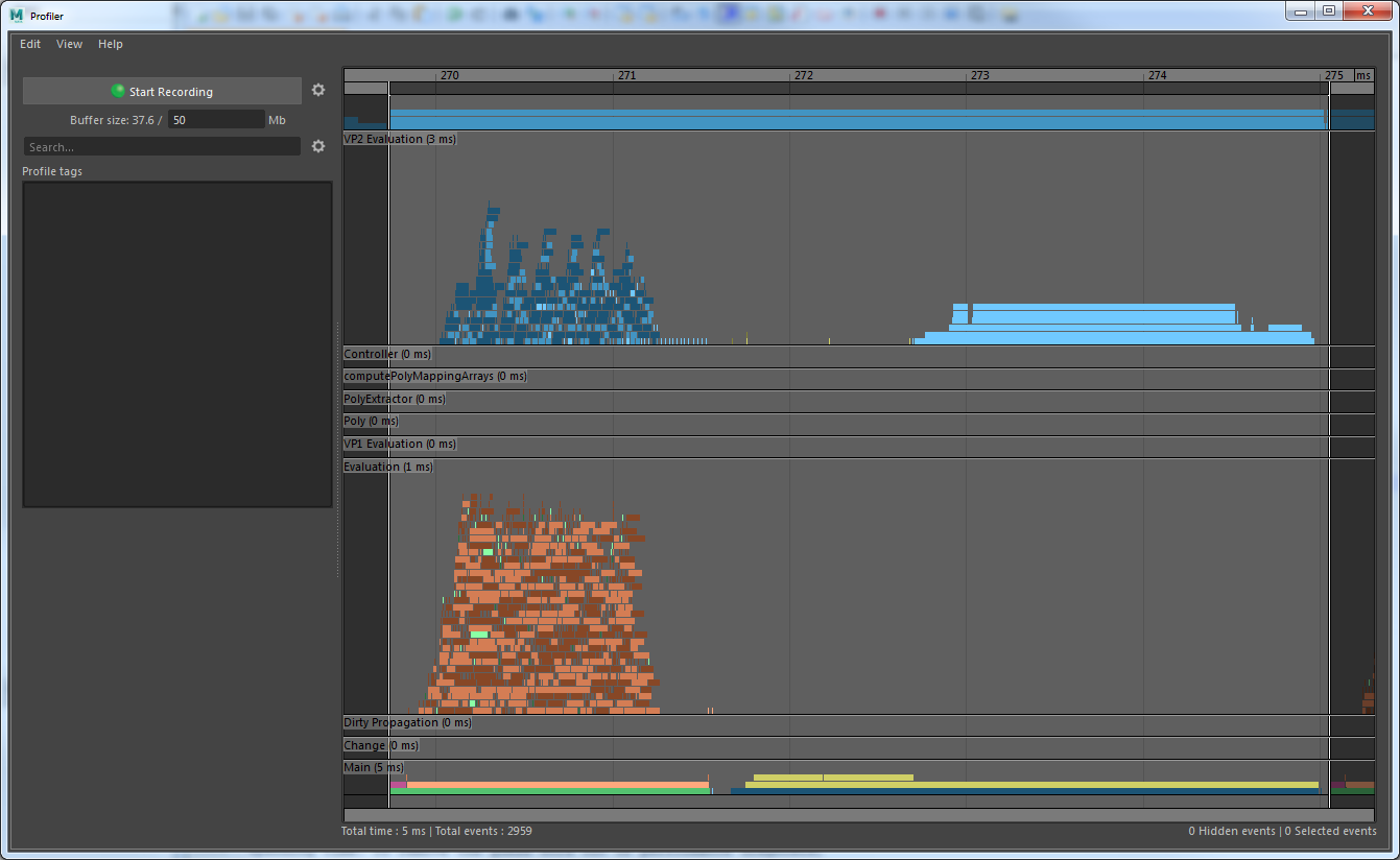
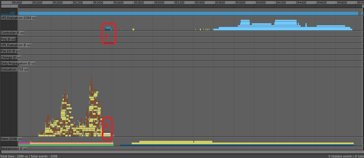
The following profiler images were created from the same scene (100 footPrintNode_GeometryOverride nodes with animated “size” attributes). In the first image Evaluation Manager Parallel Update is not enabled, and a large amount of time is spent serially preparing draw data for each footPrint node in Vp2BuildRenderLists.

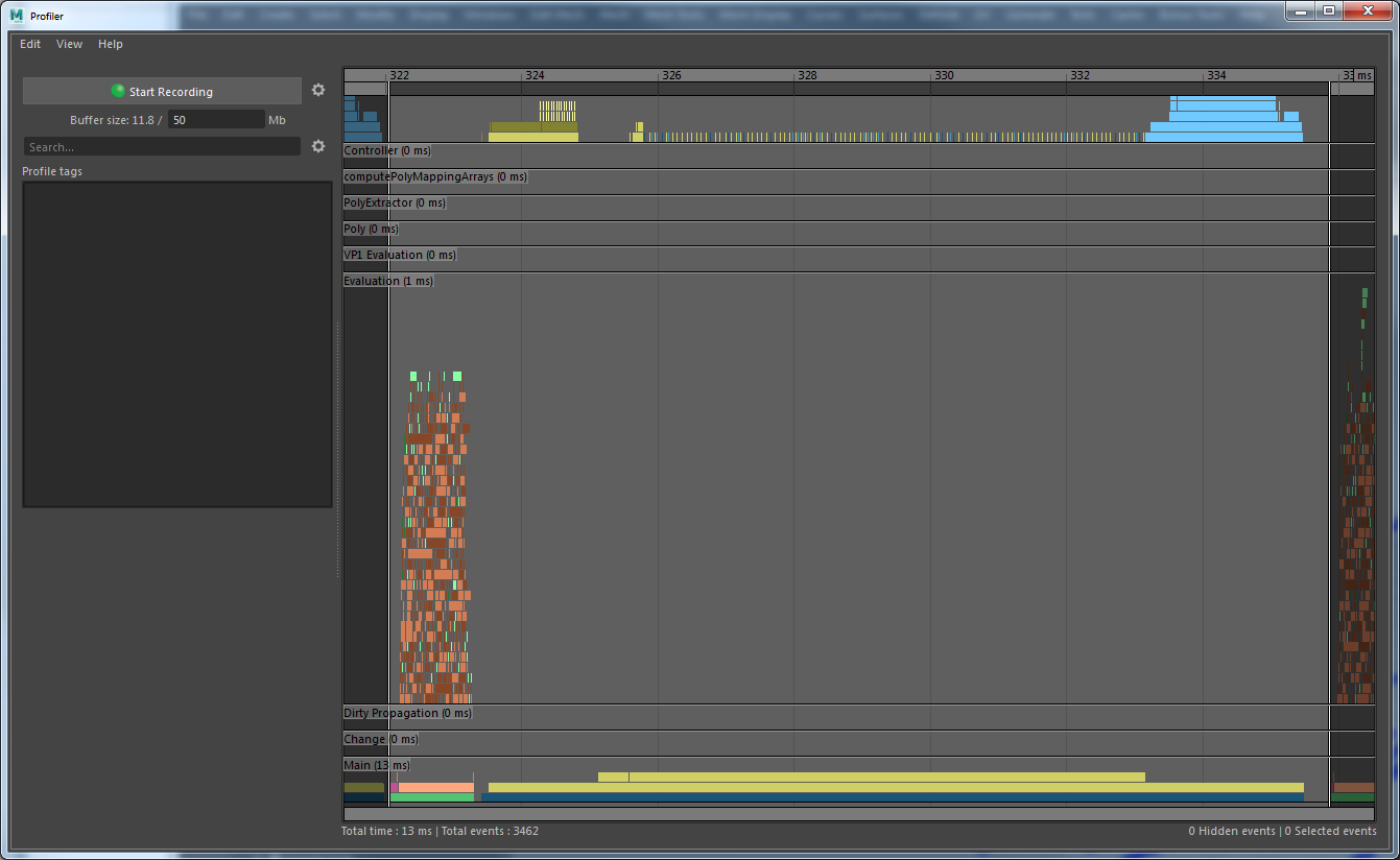
In the second image the footPrintNode_GeometryOverride has been modified to support Evaluation Manager Parallel Update. You can see that the long serial execution time in Vp2BuildRenderLists has been eliminated. All the data marshalling for VP2 is occurring in parallel while the Evaluation Manager is evaluating the Dependency Graph.

The footPrintNode_GeometryOverride example plug-in provides a detailed example for you to create an efficient MPxGeometryOverride plugin which supports Evaluation Manager Parallel Update and gives excellent performance in VP2.

Supporting Evaluation Manager Direct Update adds some restrictions to which operations can safely be performed from MPxGeometryOverride function calls. All MPxGeometryOverride functions (except cleanUp() and the destructor) may be called from a worker thread in parallel with other Maya execution. These methods must all be thread safe. An MPxGeometryOverride object is guaranteed to have at most one of its member functions called at a time. If two different MPxGeometryOverride objects “A” and “B” both require updating, then any member function on “A” could be called at the same time as any member function on “B”.

Furthermore, because these methods may be called from a worker thread, direct access to the rendering context is prohibited. MVertexBuffer and MIndexBuffer can still be used, but some of their features are prohibited from use when in Evaluation Manager Parallel Update. Details about which features are safe to use are provided in the documentation for MVertexBuffer and MIndexBuffer.

Tracking Topology

Evaluation Manager Parallel Update currently has the limitation that it can only be used on geometries that do not have animated topology. The status of whether topology is animated or not needs to be tracked from the geometry’s origin to its display shape.

If the nodes in the graph are built-in nodes, Maya can know if an animated input will affect the output geometry topology. Similarly, deformers (even custom ones derived from MPxDeformerNode), are assumed to simply deform their input in their output, keeping the same topology.

However, more generic nodes can also generate geometries. When a custom node is a MPxNode, Maya cannot know whether an output geometry has animated topology. It therefore assumes the worst and treats the topology as animated. While this approach is the safest, it can prevent optimizations such as Evaluation Manager Parallel Update.

As of Maya 2019, a new API has been added to inform Maya about attributes that might not affect the topology of an output geometry.

• The first step is to override the MPxNode::isTrackingTopology() method so that Maya can track topology information for this node.
• The second step is the use the new version of the MPxNode::attributeAffects() method to inform Maya that while the source attribute affects the output attribute, it does not affect its topology.

Using this new API helps Maya to know that it is safe to use Evaluation Manager Parallel Update and benefit from its performance boost in more situations.

Profiling Plug-ins

To visualize how long custom plug-ins take in the new profiling tools (see Profiling Your Scene) you will need to instrument your code. Maya provides C++, Python, and MEL interfaces for you to do this. Refer to the Profiling using MEL or Python or the API technical docs for more details.

Profiling Your Scene

In the past, it could be challenging to understand where Maya was spending time. To remove the guess-work out of performance diagnosis, Maya includes a new integrated profiler that lets you see exactly how long different tasks are taking.

Open the Profiler by selecting:

• Windows > General Editors > Profiler from the Maya menu
• Persp/Graph Layout from the Quick Layout buttons and choosing Panel Layout > Profiler.

Once the Profiler window is visible:

1. Load your scene and start playback
2. Click Start in the Profiler to record information in the pre-allocated record buffer.
3. Wait until the record buffer becomes full or click Stop in the Profiler to stop recording. The Profiler shows a graph demonstrating the processing time for your animation.
4. Try recording the scene in DG, Serial, Parallel, and GPU Override modes.

Tip. By default, the Profiler allocates a 20MB buffer to store results. The record buffer can be expanded in the UI or by using the profiler -b value; command, where value is the desired size in MB. You may need this for more complex scenes.

The Profiler includes information for all instrumented code, including playback, manipulation, authoring tasks, and UI/Qt events. When profiling your scene, make sure to capture several frames of data to ensure gathered results are representative of scene bottlenecks.

The Profiler supports several views depending on the task you wish to perform. The default Category View, shown below, classifies events by type (e.g., dirty, VP1, VP2, Evaluation, etc). The Thread and CPU views show how function chains are subdivided amongst available compute resources. Currently the Profiler does not support visualization of GPU-based activity.

Understanding Your Profile

Now that you have a general sense of what the Profiler tool does, let’s discuss key phases involved in computing results for your scene and how these are displayed. By understanding why scenes are slow, you can target scene optimizations.

Every time Maya updates a frame, it must compute and draw the elements in your scene. Hence, computation can be split into one of two main categories:

1. Evaluation (i.e., doing the math that determines the most up-to-date values for scene elements)
2. Rendering (i.e., doing the work that draws your scene in the viewport).

When the main bottleneck in your scene is evaluation, we say the scene is evaluation-bound. When the main bottleneck in your scene is rendering, we say the scene is render-bound.

Profiler Colors

Each event recorded by the profiler has an associated color. Each color represents a different type of event. By understanding event colors you can quickly interpret profiler results. Some colors are re-used and so have different meanings in different categories.

• Dirty Propagation (Pink and Purple)
• Pull Evaluation (Dark Green)
• Forward or Evaluation Manager Evaluation (Peach, Tan and Brown)
• Set Time (Light Green)
• Qt Events (Light Blue)
• VP2 Rendering (Light Blue)
• VP2 Pull Updates (Light and Dark Yellow and Blue)
• VP2 Push or Direct Updates (Light and Dark Blue)
• GPU Override CPU usage (Light and Dark Yellow)
• Cache Restore (Yellow)
• Cache Skipped (Gray)

We can’t see every different type of event in a single profile, because some events like Dirty Propagation only occur with Evaluation Manager off, and other events like GPU Override CPU usage only occur with Evaluation Manager on. In the following example profiles we will show DG Evaluation, Evaluation Manager Parallel Evaluation, GPU Override Evaluation, Evaluation Cached Evaluation and VP2 Cached Evaluation.
Through these examples we’ll see how to interpret a profile based on graph colors and categories, and we’ll learn how each performance optimization in Maya can impact a scene’s performance. The following example profiles are all generated from the same simple FK character playing back.

DG Evaluation

In this profile of DG Evaluation we can see several types of event.

1. Pink and purple Dirty Propagation events in the Dirty Propagation category.
2. Dark green Pull Evaluation events in the Evaluation category.
3. Blue VP2 Pull Translation and light blue VP2 Rendering in the VP2 Evaluation category.
4. Yellow events in the VP2 Evaluation category show time VP2 spent waiting for data from Dependency Graph nodes.

A significant fraction of each frame is spent on Dirty Propagation, a problem which is alleviated by Evaluation Manager.

EM Parallel Evaluation

In this profile of EM Parallel Evaluation we can see all the purple and pink dirty propagation is gone.

1. Peach, tan and brown EM Parallel Evaluation events of the FK rig colored. The high stack of events represents some evaluation occurring in parallel (use thread view to better understand parallelism).
2. Tan and brown EM Parallel Evaluation events while Maya evaluates the skin cluster to compute the deformed mesh. These events occur serially because the Dependency Graph has no parallelism.
3. Dark blue and blue VP2 Direct Update events translate data into a VP2 render-able format.
4. Yellow in the Main category and light blue in the VP2 Evaluation category are VP2 Rendering events.

In this profile we see much less time spent on Vp2SceneRender (4). This occurs because time spent reading data from dependency nodes has been moved from rendering to EM Parallel Evaluation (1). DG evaluation uses a data pull model, while EM Evaluation uses a data push model. Additionally, some geometry translation (2), is also moved from rendering to evaluation. We call geometry translation during evaluation “VP2 Direct Update”. A significant portion of each frame is spent deforming and translating the geometry data, a problem which is alleviated by GPU Override.

EM Parallel Evaluation with GPU Override

In this profile of EM Parallel Evaluation we can see one major new difference from the previous profile of EM Parallel Evaluation.

1. Light and dark yellow GPU Override events have replaced the long serial central part of the EM Parallel Evaluation profile (2 & 3 from EM Parallel Evaluation). The GPU Override events represent the time taken on the CPU to marshal data and launch the GPU computation.
2. Peach, tan and brown EM Parallel Evaluation events here have roughly the same duration as EM Parallel Evaluation even though the relative size of the rig evaluation events with GPU Override is larger. This is because the scale of this profile is different from the scale of the previous profile. In the profile of EM Parallel Evaluation with GPU Override the total time displayed is about 5ms. In the previous profile of EM Parallel Evaluation the total time displayed is about 12ms.
3. Light blue VP2 Render events have experienced a similar relative stretching (2).

EM Evaluation Cached Playback

In this profile of EM Evaluation Cached Playback we can see several new types of event.

1. Yellow Restore Cache events recording the time taken to update each FK rig node which has cached data. There are also brown VP2 Direct Update events used to track update of the VP2 representation of the data.
2. Yellow Restore Cache event for the deformed mesh. This represents the time taken to restore the data into the Maya node, and to translate the data into VP2 for drawing using VP2 Direct Update.

EM VP2 Hardware Cached Playback

1. Dark blue VP2 Hardware Cache Restore events have replaced the long serial Cache Restore event (2 from EM Evaluation Cached Playback). Restoring the VP2 Hardware Cache is much faster because the data is already in in the render-able format and stored on the GPU.
2. Gray Cache Skipped event signaling data in the dependency node is not updated.

Evaluation-Bound Performance

When the main bottleneck in your scene is evaluation, we say the scene is evaluation-bound. There are several different problems that may lead to evaluation-bound performance.

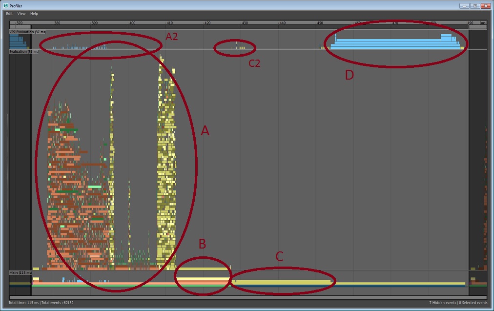
Lock Contention. When many threads try to access a shared resource you may experience Lock Contention, due to lock management overhead. One clue that this may be happening is that evaluation takes roughly the same duration regardless of which evaluation mode you use. This occurs since threads cannot proceed until other threads are finished using the shared resource.

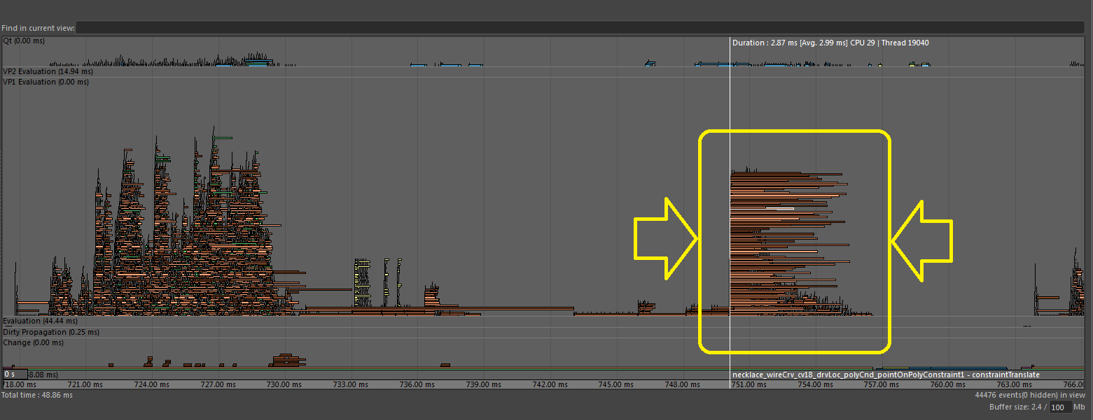
Here the Profiler shows many separate identical tasks that start at nearly the same time on different threads, each finishing at different times. This type of profile offers a clue that there might be some shared resource that many threads need to access simultaneously.

Below is another image showing a similar problem.

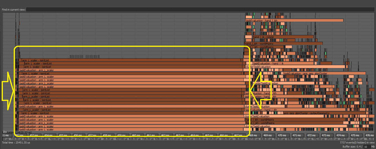
In this case, since several threads were executing Python code, they all had to wait for the Global Interpreter Lock (GIL) to become available. Bottlenecks and performance loses caused by contention issues may be more noticeable when there is a high concurrency level, such as when your computer has many cores.

If you encounter contention issues, try to fix the code in question. For the above example, changing node scheduling converted the above profile to the following one, providing a nice performance gain. For this reason, Python plug-ins are scheduled as Globally Serial by default. As a result, they will be scheduled one after the other and will not block multiple threads waiting for the GIL to become available.

Clusters. As mentioned earlier, if the EG contains node-level circular dependencies, those nodes will be grouped into a cluster which represents a single unit of work to be scheduled serially. Although multiple clusters may be evaluated at the same time, large clusters limit the amount of work that can be performed simultaneously. Clusters can be identified in the Profiler as bars wiip.opaqueTaskEvaluation label, shown below.

If your scene contains clusters, analyze your rig’s structure to understand why circularities exist. Ideally, you should strive to remove coupling between parts of your rig, so rig sections (e.g., head, body, etc.) can be evaluated independently.

Tip. When troubleshooting scene performance issues, you can temporarily disable costly nodes using the per-node frozen attribute. This removes specific nodes from the EG. Although the result you see will change, it is a simple way to check that you have found the bottleneck for your scene.

Render-Bound Performance

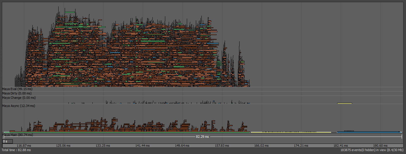
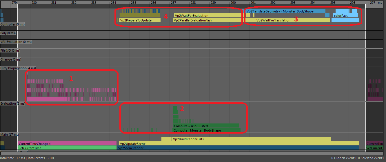
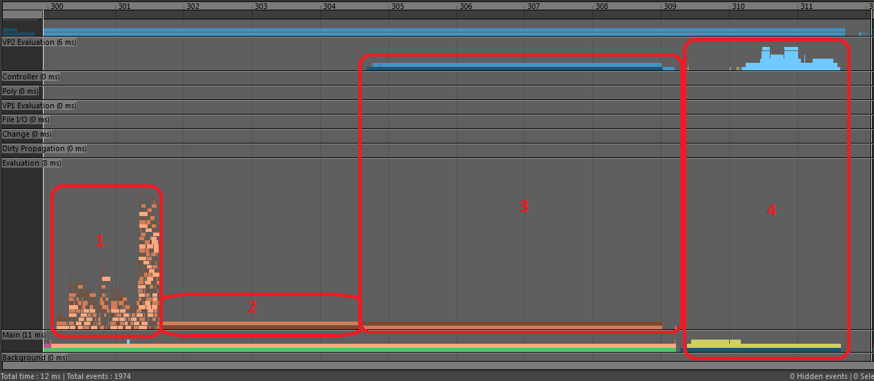
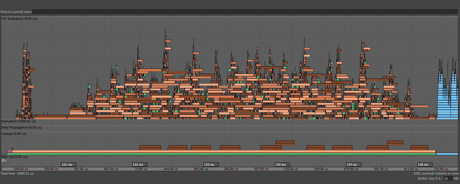
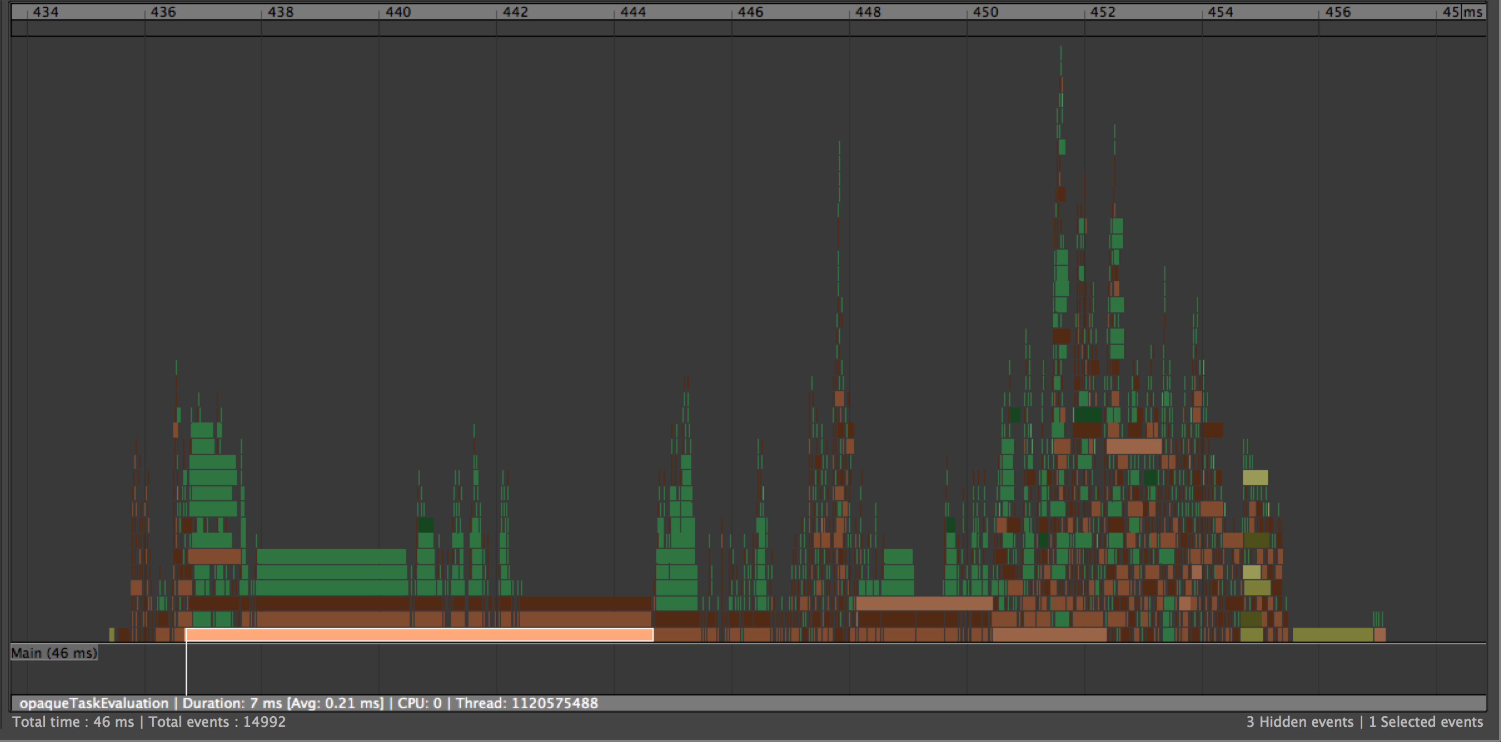
When the main bottleneck in your scene is rendering, we say the scene is render-bound. The following is an illustration of a sample result from the Maya Profiler, zoomed to a single frame measured from a large scene with many animated meshes. Because of the number of objects, different materials, and the amount of geometry, this scene is very costly to render.

The attached profile has four main areas:

• Evaluation (A)
• GPUOverridePostEval (B)
• Vp2BuildRenderLists (C)
• Vp2Draw3dBeautyPass (D)

In this scene, a substantial number of meshes are being evaluated with GPU Override and some profiler blocks appear differently from what they would otherwise.

Evaluation. Area A depicts the time spent computing the state of the Maya scene. In this case, the scene is moderately well-parallelized. The blocks in shades of orange and green represent the software evaluation of DG nodes. The blocks in yellow are the tasks that initiate mesh evaluation via GPU Override. Mesh evaluation on the GPU starts with these yellow blocks and continues concurrently with the other work on the CPU.

An example of a parallel bottleneck in the scene evaluation appears in the gap in the center of the evaluation section. The large group of GPU Override blocks on the right depend on a single portion of the scene and must wait until that is complete.

Area A2 (above area A), depicts blue task blocks that show the work that VP2 does in parallel to the scene evaluation. In this scene, most of the mesh work is handled by GPU Override so it is mostly empty. When evaluating software meshes, this section shows the preparation of geometry buffers for rendering.

GPUOverridePostEval. Area B is where GPU Override finalizes some of its work. The amount of time spent in this block varies with different GPU and driver combinations. At some point there will be a wait for the GPU to complete its evaluation if it is heavily loaded. This time may appear here or it may show as additional time spent in the Vp2BuildRenderLists section.

Vp2BuildRenderLists. Area C. Once the scene has been evaluated, VP2 builds the list of objects to render. Time in this section is typically proportional to the number of objects in the scene.

Vp2PrepareToUpdate. Area C2, very small in this profile. VP2 maintains an internal copy of the world and uses it to determine what to draw in the viewport. When it is time to render the scene, we must ensure that the objects in the VP2 database have been modified to reflect changes in the Maya scene. For example, objects may have become visible or hidden, their position or their topology may have changed, and so on. This is done by VP2 Vp2PrepareToUpdate.

Vp2PrepareToUpdate is slow when there are shape topology, material, or object visibility changes. In this example, Vp2PrepareToUpdate is almost invisible since the scene objects require little extra processing.

Vp2ParallelEvaluationTask is another profiler block that can appear in this area. If time is spent here, then some object evaluation has been deferred from the main evaluation section of the Evaluation Manager (area A) to be evaluated later. Evaluation in this section uses traditional DG evaluation.

Common cases for which Vp2BuildRenderLists or Vp2PrepareToUpdate can be slow during Parallel Evaluation are:

• Large numbers of rendered objects (as in this example)
• Mesh topology changes
• Object types, such as image planes, requiring legacy evaluation before rendering
• 3rd party plug-ins that trigger API callbacks

Vp2Draw3dBeautyPass. Area D. Once all data has been prepared, it is time to render the scene. This is where the actual OpenGL or DirectX rendering occurs. This area is broken into subsections depending on viewport effects such as depth peeling, transparency mode, and screen space anti-aliasing.

Vp2Draw3dBeautyPass can be slow if your scene:

• Has Many Objects to Render (as in this example).
• Uses Transparency. Large numbers of transparent objects can be costly since the default transparency algorithm makes scene consolidation less effective. For very large numbers of transparent objects, setting Transparency Algorithm (in the vp2 settings) to Depth Peeling instead of Object Sorting may be faster. Switching to untextured mode can also bypass this cost
• Uses Many Materials. In VP2, objects are sorted by material prior to rendering, so having many distinct materials makes this time-consuming.
• Uses Viewport Effects. Many effects such as SSAO (Screen Space Ambient Occlusion), Depth of Field, Motion Blur, Shadow Maps, or Depth Peeling require additional processing.

Other Considerations. Although the key phases described above apply to all scenes, your scene may have different performance characteristics.

For static scenes with limited animation, or for non-deforming animated objects, consolidation is used to improve performance. Consolidation groups objects that share the same material. This reduces time spent in both Vp2BuildRenderLists and Vp2Draw3dBeatyPass, since there are fewer objects to render.

Saving and Restoring Profiles

Profile data can be saved at any time for later analysis using the Edit -> Save Recording... or Edit -> Save Recording of Selected Events... menu items in the Profiler window. Everything is saved as plain string data (see the appendix describing the profiler file format for a description of how it is stored) so that you can load profile data from any scene using the Edit -> Load Recording... menu item without loading the scene that was profiled.

Troubleshooting Your Scene

Analysis Mode

The purpose of Analysis Mode is to perform more rigorous inspection of your scene to catch evaluation errors. Since Analysis Mode introduces overhead to your scene, only use this during debugging activities; animators should not enable Analysis Mode during their day-to-day work. Note that Analysis Mode is not thread-safe, so it is limited to Serial; you cannot use analysis mode while in Parallel evaluation.

The key function of Analysis Mode is to:

• Search for errors at each playback frame. This is different than Safe Mode, which only tries to identify problems at the start of parallel execution.
• Monitor read-access to node attributes. This ensures that nodes have a correct dependency structure in the EG.
• Return diagnostics to better understand which nodes influence evaluation. This is currently limited to reporting one destination node at a time.

Tip. To activate Analysis Mode, use the dbtrace -k evalMgrGraphValid; MEL command.

Once active, error detection occurs after each evaluation. Missing dependencies are saved to a file in your machine’s temporary folder (e.g., %TEMP%\_MayaEvaluationGraphValidation.txt on Windows). The temporary directory on your platform can be determined using the internalVar -utd; MEL command.

To disable Analysis Mode, type: dbtrace -k evalMgrGraphValid -off;

Let’s assume that your scene contains the following three nodes. Because of the dependencies, the evaluation manager must compute the state of nodes B and C prior to calculating the state of A.

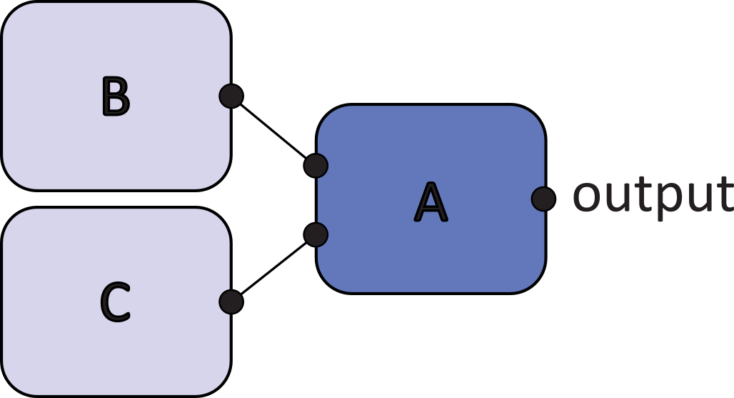
Now let’s assume Analysis Mode returns the following report:

Detected missing dependencies on frame 56
{
     A.output <-x- B
     A.output <-x- C [cluster]
}
Detected missing dependencies on frame 57
{
    A.output <-x- B
    A.output <-x- C [cluster]
}

The <-x- symbol indicates the direction of the missing dependency. The [cluster] term indicates that the node is inside of a cycle cluster, which means that any nodes from the cycles could be responsible for attribute access outside of evaluation order

In the above example, B accesses the output attribute of A, which is incorrect. These types of dependency do not appear in the Evaluation Graph and could cause a crash when running an evaluation in Parallel mode.

There are multiple reasons that missing dependencies occur, and how you handle them depends on the cause of the problem. If Analysis Mode discovers errors in your scene from bad dependencies due to:

• A user plug-in. Revisit your strategy for managing dirty propagation in your node. Make sure that any attempts to use “clever” dirty propagation dirty the same attributes every time. Avoid using different notification messages to trigger pulling on attributes for computation.
• A built-in node. You should communicate this information to us. This may highlight an error that we are unaware of. To help us best diagnose the causes of this bug, we would appreciate if you can provide us with the scene that caused the problem.

Graph Execution Order

There are two primary methods of displaying the graph execution order.

The simplest is to use the ‘compute’ trace object to acquire a recording of the computation order. This can only be used in Serial mode, as explained earlier. The goal of compute trace is to compare DG and EM evaluation results and discover any evaluation differences related to a different ordering or missing execution between these two modes.

Keep in mind that there will be many differences between runs since the EM executes the graph from the roots forward, whereas the DG uses values from the leaves. For example in the simple graph shown earlier, the EM guarantees that B and C will be evaluated before A, but provides no information about the relative ordering of B and C. However in the DG, A pulls on the inputs from B and C in a consistent order dictated by the implementation of node A. The EM could show either "B, C, A" or "C, B, A" as their evaluation order and although both might be valid, the user must decide if they are equivalent or not. This ordering of information can be even more useful when debugging issues in cycle computation since in both modes a pull evaluation occurs, which will make the ordering more consistent.

The Evaluation Toolkit

A set of debugging tools used to be shipped as a special shelf in Maya Bonus Tools, but they are now built-in within Maya. The Evaluation Toolkit provides features to query and analyze your scene and to activate / deactivate various modes. See the accompanying Evaluation Toolkit documentation for a complete list of all helper features.

Known Limitations

This section lists known limitations for the new evaluation system.

• VP2 Motion Blur will disable Parallel evaluation. For Motion Blur to work, the scene must be evaluated at different points in time. Currently the EM does not support this.
• Scenes using FBIK will revert to Serial. For several years now, Autodesk has been deprecating FBIK. We recommend using HIK for full-body retargeting/solving.
• dbtrace will not work in Parallel mode. As stated in the Analysis Mode section, the dbtrace command only works in Serial evaluation. Having traces enabled in Parallel mode will likely cause Maya to crash.
• The DG Profiler crashes in Parallel Mode. Unless you are in DG evaluation mode, you will be unable to use the legacy DG profiler. Time permitting, we expect to move features of the DG profiler into the new thread-safe integrated profiler.
• Batch rendering scenes with XGen may produce incorrect results.
• Evaluation manager in both Serial and Parallel mode changes the way attributes are cached. This is done to allow safe parallel evaluation and prevent re-computation of the same data by multiple threads. This means that some scenes may evaluate differently if multiple computations of the same attribute occur in one evaluation cycle. With the Evaluation Manager, the first value will be cached.
• VP2 Direct update does not work with polySoftEdge nodes.

Appendices

Profiler File Format

The profiler stores its recording data in human-readable strings. The format is versioned so that older format files can still be read into newer versions of Maya (though not necessarily vice-versa).

This is a description of the version 1 format.

First, a content example:

1     #File Version, # of events, # of CPUs
2     2\t12345\t8
3     Main\tDirty
4     #Comment mapping---------
5*    @27 = MainMayaEvaluation
6     #End comment mapping---------
7     #Event time, Comment, Extra comment, Category id, Duration, \
          Thread Duration, Thread id, Cpu id, Color id
8*    1234567\t@12\t@0\t2\t12345\t11123\t36\t1\t14
9     #Begin Event Tag Mapping---------
10    #Event ID, Event Tag
11*   123\tTaggy McTagface
12    #End Event Tag Mapping---------
13    #Begin Event Tag Color Mapping---------
14    #Tag Label, Tag Color
15*   Taggy\tMcTagface\t200\t200\t13
16    #End Event Tag Color Mapping---------
EOF

The following table describes the file format structure by referring to the previous content:

Sample version 2 file on 4 CPUs containing a single event of type “ETName”, description “ETDescription”, in category “ETCategory” with description “Category description”, using color 7, of duration 100 ticks, starting at tick 999, on a single thread with ID 22, tagged with “TagMe” which has color red (255 0 0)

#File Version, # of events, # of CPUs
2   1   4
ETCategory
Category description
#Comment mapping---------
@0 = ETName
#End comment mapping---------
999 @0  @0  1   100 100 22  1   7
#Begin comment description mapping---------
@1 = ETDescription
#End comment description mapping---------
#Begin Event Tag Mapping---------
#Event ID, Event Tag
1   TagMe
#End Event Tag Mapping---------
#Begin Event Tag Color Mapping---------
#Tag Label, Tag Color
TagMe   255 0 0
#End Event Tag Color Mapping---------

Debugging Commands

Several commands can be used to help display information about your scene to help in debugging or optimizations. This is a summary of some of the more common ones, and represents only the available runtime information. Consult the command documentation in Maya’s online technical documentation for more information about each command.

dbcount

Maintains embedded code location counters for higher-level debugging of scene operation. Generally, this uses specialized code that is only available in custom builds.

Synopsis: dbcount [flags]
Flags:
   -e -enabled      on|off
   -f -file         String
   -k -keyword      String
   -l -list        
  -md -maxdepth     UnsignedInt
   -q -quick       
   -r -reset       
   -s -spreadsheet

Command Type: Command

dbmessage

Monitors messaging that adds and removes DAG and DG nodes.

Synopsis: dbmessage [flags]
Flags:
   -f -file     String
   -l -list    
   -m -monitor  on|off
   -t -type     String

Command Type: Command

dbtrace

Turns on conditional code, typically to print out status information or to take different code paths when enabled.

To find available trace objects use dbtrace –q to list currently-enabled traces, and dbtrace –q –off to list currently-disabled traces.

To find the current trace output target, use dbtrace -q -k keyword -o.

See below for information on specific keywords.

Note: Work is currently in progress to make these trace objects more flexible. It is a current design constraint that sometimes they are visible in a release, even though they only function internally, and some cannot be used when using Parallel evaluation.

Synopsis: dbtrace [flags]
Flags:
   -q -query
   -f -filter   String
   -i –info
   -k -keyword  String (multi-use)
              (Query Arg Optional)
   -m -mark    
   -o -output   String
 -off -        
   -t -title    String
  -tm -timed    on|off
   -v -verbose

Command Type: Command

dgdebug

Historical debugging command; not robust or documented. Deprecated: Use the newer dbpeek command.

No help is provided for this command.

dgdirty

Forces dirty/clean states onto specified plugs and everything downstream from them. Meant to be a safety net for restoring proper states to your scene when something has gone wrong.

You should not need to use this command, but it will continue to exist as a “reset button”, just in case.

Synopsis: dgdirty [flags] [String...]
Flags:
   -q -query
   -a -allPlugs    
   -c -clean       
   -i -implicit    
   -l -list         String
   -p -propagation
  -st -showTiming  
   -v -verbose     

Command Type: Command

dgeval

Forces the node to compute certain plugs. Like dgdirty, this command is meant to be a safety net if computation has not occurred in the proper order. Similar in function to the getAttr command, but since it returns no results, it can handle all attribute types, not only those supported by getAttr.

Synopsis: dgeval [flags] String...
Flags:
 -src -        
   -v -verbose

Command Type: Command

dgInfo

Dumps information about the current state of the graph. Be aware that when plug dirty states are reported, they represent the connection associated with the plug. In fan-out or in-out connections there will be more than one dirty state associated with the connection attached to the plug. This means it is legal to see A->B as dirty but B->A as clean if A has multiple connections. Being Deprecated: Use the newer dbpeek command.

Synopsis: dgInfo [flags] [String...]
Flags:
 -all -allNodes     
   -c -connections  
   -d -dirty         on|off
   -n -nodes        
  -nd -nonDeletable
  -nt -type          String
  -of -outputFile    String
   -p -propagation   on|off
   -s -short        
 -sub -subgraph     
  -sz -size         

Command Type: Command

dgmodified

Checks on the reason a file requests saving when no changes have been made.

Synopsis: dgmodified

No Flags.

dbpeek

This command is called out intentionally, as it combines multiple operations into a single command by use of various operations.

It runs one of several operations that provide a view into the data internals in the scene. This is the most useful and flexible of the debugging commands, and new variations of it are often being introduced. Use dbpeek -q -op to show a list of currently available operations and dbpeek -op X -q to show detailed help for operation X.

See below for information on specific keywords.

Note: The syntax of the argument flag allows for both keyword argument=’key’ and keyword/value argument=’key=value’ forms.

Synopsis: dbpeek [flags] [String...]
Flags:
   -q -query
   -a -argument         String (multi-use) (Query Arg Mandatory)
 -all -allObjects      
   -c -count            UnsignedInt
  -eg -evaluationGraph
  -of -outputFile       String
  -op -operation        String (Query Arg Optional)

Command Type: Command

dbpeek -op attributes

Analyzes node or node-type attributes and dumps information about them based on what the selected operation type.

Various arguments to the operation change the content of the output. The essence remains the same; the attributes belong to the node or node type.

If no nodes are selected, then this command prints the list of all attributes on all nodes. For example, if you had a node type called reversePoint with a vector input and a vector output.

type=detail would output this JSON data:

{
    "nodes" :
    {
      "reversePoint" :
      {
        "staticAttributes" : [
          { "pointInput" : [
              "pointInputX",
              "pointInputY",
              "pointInputZ",
            ]
          },
          { "pointOutput" :
            [
15">              "pointOutputX",
              "pointOutputY",
              "pointOutputZ",
            ]
          }
        ],
        "extensionAttributes" : []
      }
    }
  }

type=affects would output this DOT data:

digraph G
{
    compound=true;
    subgraph cluster_NODENAME
    {
        label="Node NODENAME, Type NODETYPE";
        color=".7 .0 .0";
        ia [label="ia/inputAttribute",style="rounded",shape=ellipse];
        oa [label="oa/outputAttribute",style="rounded",shape=rectangle];
        ia -> oa;
    }
}

and type=validate would output this JSON validation summary:

{
  "Attribute Validation" :
  {
    "NODENAME" :
    {
      "staticAttributes" :
      [
        {
          "Both input and output attributes in compound" :
          [
            { "root" : "rootAttribute",
              "inputs" : ["inputChild"],
              "outputs" : ["outputChild"],
            }
          ]
        }
      ]
    }
  }
}

dbpeek -op cache

This operation is explained in detail in the Debugging section of the Maya Cached Playback whitepaper.

dbpeek -op cmdTracking

By default, when no detail argument is present it shows a list of all commands run since the last reset as well as a count of how many of each type were executed.

Outputs in command/count pair form, one per line, with a tab character separating them.

dbpeek -op connections

By default, when no type argument is present, shows a list of all connections in the DG.

dbpeek -op data

Dumps the current contents of a node’s plug data in a standard format. By default the output is in CSV format consisting of 5 columns: NODE PLUG DATA_TYPE CLEAN_STATE DATA_AS_TEXT

Example for a simple integer attribute with a dirty value of 5: MyNode MyPlug Int32 0 5

dbpeek -op context

Analyzes context evaluation to detect various errors violating the design.

Sample output for isolation tests:

{
    "context isolation": {
        "frame": 5.0,
        "type": "animatedNodes",
        "verbose": true,
        "errors": [
            {
                "node": "ikHandle1",
                "type": "ikHandle",
                "attribute": "ikFkManipulation",
                "call stack": [
                    "METHOD Line NUMBER",
                    "METHOD Line NUMBER",
                    "METHOD Line NUMBER"
                ]
            },
            {
                "node": "shape",
                "type": "mesh",
                "attribute": "displaySmoothMesh",
                "call stack": [
                    "METHOD Line NUMBER",
                    "METHOD Line NUMBER",
                    "METHOD Line NUMBER"
                ]
            }
        ],
        "time out": true
    }
}

Sample output for correctness tests:

{
    "context correctness": {
        "frame": 14.0,
        "verbose": true,
        "errors": [
            {
                "node": "IKSpineCurveShape",
                "type": "nurbsCurve",
                "attributes": [
                    "worldSpace"
                ]
            }
        ],
        "failed to compare": [
            "input",
            "clusterXforms",
            "clusterTransforms",
            "target",
            "mySpecialAttribute"
        ],
        "time out": true
    }
}

dbpeek -op edits

Shows a list of all nodes for which tracking is currently enabled. The “track” flag is mandatory.

dbpeek -op evalMgr

Outputs the current state of all of the custom evaluators used by the Evaluation Manager.

dbpeek -op graph

Gets a list of nodes or connections from either the dependency graph or the underlying evaluation graph.

dbpeek -op mesh

Dumps the current contents of the mesh to a standard format. There are two types of formatting and two levels of detail to present.

For the default level of detail, the default CSV format output will look like this:

NODE_NAME,DATA_TYPE,DATA_COUNT

For example, a cube containing 32 vertices would have these lines:

Node,DataType,Count
pCubeShape1,outMesh,32

The JSON equivalent format would look like this:

{
    "pCubeShape1" : {
        "outMesh" : "32"
    }
}

If the full detail is requested, then the (abbreviated) output for CSV format will look like this:

Node,Plug,Clean,Value
pCubeShape1,outMesh[0],1,0.0 0.0 0.0
pCubeShape1,outMesh[1],1,0.0 0.5 0.0
...
pCubeShape1,outMesh[32],1,1.0 1.0 1.0

and like this for JSON format:

{
    "pCubeShape1" : {
        "outMesh" : {
            "clean" : 1,
            "0" : [0.0, 0.0, 0.0],
            "1" : [0.0, 0.5, 0.0],
            "..." : "...",
            "32": [1.0, 1.0, 1.0]
        }
    }
}

dbpeek -op metadata

Shows node metadata. The default operation shows a list of all nodes containing metadata.

dbpeek -op node

Show select debugging information on DG nodes. See also the “plug” and “connection” operations for display of information specific to those facets of a node. If no arguments are used then the ones marked as [default] will all be enabled, for convenience.

dbpeek -op nodes

By default, when no detail argument is present, shows a list of all currently registered node types.

dbpeek -op nodeTracking

By default, when no argument is present, shows a list of all nodes created since the last reset along with a count of how many of each type were created. Output is in the form of nodeType/count pairs, one per line, with a tab character separating them.

dbpeek -op plugs

Shows information about all of the plugs in a scene. By default, when no argument is present, shows static plug footprint. A lot of this is only displayed in specially-instrumented builds, and generally only of use internally.

Revisions

2020

• Updated the dbtrace section to add info about:
  • OGSPolyGhosts
  • cacheConfig
  • evalMgr
  • evalMgrGraphInvalid
  • peekCache
  • peekContext
• Added a link in the dbpeek section to details regarding the new cache operation.

2019

• Updated the Key Concepts section.
  • Added more info about the different graphs (DG, EG, SG).
• Added a section about VP2 Integration and Evaluation Manager Parallel Update.
• Added a section about Tracking Topology for Evaluation Manager Parallel Update.
• Updated the Custom Evaluators section to describe the new evaluators.
  • New evaluators:
    • curveManager (now with its own subsection)
    • cache
    • cycle

2018

• Created an Appendices section.
  • Added a section that describes the Profiler File Format.
  • Moved Debugging Commands section to the Appendices.
• Updated the Custom Evaluators section to describe the new evaluators.
  • New evaluators:
    • curveManager
    • hik
  • Added information on isolate-select and expressions to the Invisibility Evaluator
  • Added new deformer types supported in GPU override:
    • deltaMush
    • lattice
    • nonLinear
    • tension

2017

• Added section on graph invalidation.
• Added information about different ways to query scheduling information (see Thread Safety).
• Updated the Custom Evaluators section to describe the new evaluators.
  • New evaluators:
    • invisibility
    • frozen
    • timeEditorCurveEvaluator
  • dynamics evaluator support for Parallel evaluation of scenes with dynamics is now enabled by default.
• Added Custom Evaluator API section.
• Added Evaluation Toolkit section.
• Added Debugging Commands section.
• Miscellaneous typo fixes and small corrections.

2016 Extension 2

• Added tip about the controller command.
• Updated Other Evaluators subsection in the Custom Evaluators section to describe the new evaluators.
  • New evaluators:
    • transformFlattening
    • reference
  • deformer evaluator is now enabled by default.
  • dynamics evaluator has a new behavior, disabled by default, to support Parallel evaluation of scenes with dynamics.
• Updated Evaluator Conflicts subsection in the Custom Evaluators section.
• Updated Python plug-ins scheduling to Globally Serial.
• Updated Render-Bound Performance subsection in the Profiling Your Scene section.
• Added new images for graph examples.
• Miscellaneous typo fixes and small corrections.

2016

• Initial version of the document.